What is Composite curing? Composite curing is a critical thermal and chemical process that transforms a mixture of fibers and a polymer matrix into a rigid fiber-reinforced composite. Through controlled temperature and pressure cycles, curing induces molecular cross-linking, which is essential for achieving the material’s final structural integrity and mechanical performance.
Without precise thermal management, these materials fail to meet the rigorous demands of real-world engineering applications. Because optimizing these parameters experimentally is costly, engineers increasingly rely on advanced computational methods to design effective thermal cycles.
Here at CAE Assistant, this comprehensive guide details the core fundamentals of fiber-reinforced composites and examines standard curing methodologies used in modern manufacturing. Furthermore, we demonstrate how to leverage Abaqus simulation software—specifically utilizing custom Fortran subroutines—to accurately model the composite curing process. This provides engineers, researchers, and students with a practical framework to optimize curing cycles, improve composite quality, and reduce production defects.
To ensure the model can properly address the needs of a wide range of users—from beginners to advanced industrial applications requiring high accuracy—various material models have been implemented and developed within these subroutines, including linear elastic instantaneously hardening (Chile), path-dependent, and viscoelastic models.
What are fiber-reinforced composites (FRCs)?
Fiber-reinforced composites are a class of materials consisting of two main phases: reinforcing fibers (phase 1) embedded within a matrix (phase 2). However, some references consider the interface between the matrix and fiber as a separate phase. Figure 1 depicts a piece of fiber-reinforced composite.
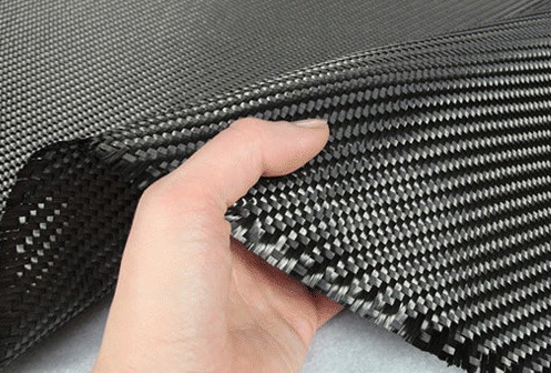
Figure 1: A piece of fiber-reinforced composite
The fibers in FRCs are typically made of stiff materials to provide sufficient strength for the composite. The matrix, often a type of polymer, holds the fibers together and transfers stress between them. When these two components are combined, a composite with unique properties is formed. This composite is lightweight yet strong. So, it is suitable for various applications.
Common types of FRCs
Fiber-reinforced composite (FRC) is a general term that represents a wide range of materials with diverse properties. Depending on the characteristics of the fibers and matrix, FRCs can be classified into various types. Each type, with its distinct properties, is ideal for specific applications.
Figure 2 presents a classification of FRCs based on their matrix material. As shown, FRCs can be made from various matrices, including polymers, metals, ceramics, and carbon/carbon materials. Among these, polymer matrix FRCs are the most widely used composites. They can be further divided into two subgroups: thermoplastics and thermosets.
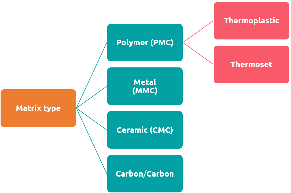
Figure 2: A classification of composites based on their matrix material
Thermoplastics are a type of polymer-based matrix that can be remelted after curing. In contrast, thermosets remain permanently cured once heated. Figure 3 compares the behavior of thermoplastic and thermoset matrices when reheated after curing.
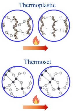
Figure 3: Comparison of the behavior of thermoplastic and thermoset matrices upon reheating
Thermosets form an extensive group of FRCs with various types and applications. Figure 4 provides a classification of thermoset composites based on the matrix and fiber materials, highlighting their diversity. While this post has focused on thermoset composites, thermoplastic composites also play a significant role in the FRC industry.
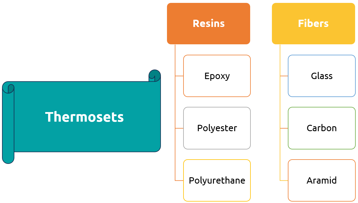
Figure 4: A classification of thermoset composites based on the matrix and fiber materials
| Explore our comprehensive Abaqus tutorial page, featuring free PDF guides and detailed videos for all skill levels. Discover both free and premium packages, along with essential information to master Abaqus efficiently. Start your journey with our Abaqus tutorial now! |
What is the composite curing process?
Curing is the process of applying heat and pressure to a composite, causing the matrix to lose its flow ability. The composite curing process must be carefully controlled to achieve the desired performance and quality in the final composite.
Today, three well-established methods are commonly used for the composite curing process: autoclave, oven curing, and heated die curing (pultrusion). In general, oven-curing is a traditional method, that utilizes a standard oven to apply heat to the composite. As depicted in Figure 5, it needs a vacuum bag to apply pressure and remove the air. Despite its lower cost compared to the autoclave method, oven curing results in higher porosity and lower mechanical properties.
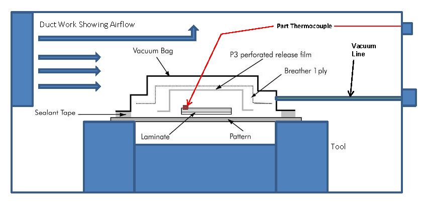
Figure 5: Schematic representation of the oven-curing process [Ref.]
The autoclave method is more advanced than the oven-curing. It utilizes a pressure vessel (autoclave) to apply both heat and pressure simultaneously to the composite, as shown in Figure 6. This process enables the production of high-quality laminates with low porosity and superior mechanical properties. However, unlike oven curing, the autoclave method is more expensive and requires complex equipment.
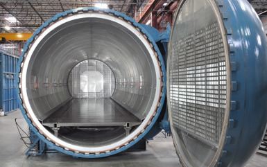
Figure 6: An autoclave device [Ref.]
Heated die curing, particularly in the context of pultrusion, offers several advantages over traditional oven and autoclave curing methods, especially for continuous composite manufacturing. For example, unlike oven and autoclave curing, which are batch processes, pultrusion with a heated die (figure 7) enables continuous production. Moreover, since heat is applied directly to the material through the die, heat loss is minimized, leading to reduced curing time. Additionally, the die not only heats but also shapes the part during curing, resulting in excellent dimensional accuracy and surface finish without the need for secondary machining. Therefore, this method can be considered a cost-effective and high-quality approach to composite curing.
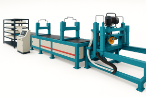
Figure 7: A pultrusion machine
How the composite curing process affects the product quality?
During the composite curing process, FRCs experience specific pressure and temperature cycles to achieve optimal quality. However, the standard composite curing process can last several hours, making it inefficient for industrial production. Manufacturers prefer to shorten the curing cycles by applying higher temperatures within shorter time periods. While this approach can increase production speed, it may impact the product quality and lead to residual deformations. Figure 8 showcases a product that experienced residual deformations after the composite curing process.
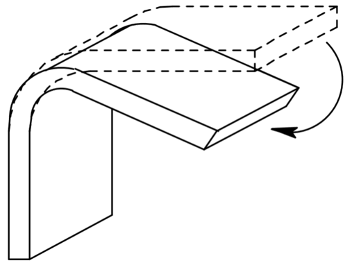
Figure 8: Schematic representation of the residual deformations in a composite [Ref.]
The traditional approach for balancing production efficiency and quality involves performing several experimental cure cycles for each product. However, the process is both costly and time-consuming. This highlights the challenge of designing optimal cure cycles that ensure both production quality and efficiency. Composite curing simulation is one way to address this challenge.
Fiber reinforced composite curing simulation
Numerical methods have simplified the fiber reinforced composite curing simulation. They are valuable alternatives to experimental tests for designing cure cycles. Such methods simplify the process of designing optimal curing cycles that ensure desired product quality while maintaining efficient production. A fiber reinforced composite curing simulation must address the coupled chemical, thermal, and mechanical fields simultaneously. So, it is referred to as the thermo-chemo-mechanical composite curing simulation.
Simulation of the thermo-chemical reactions in the curing process
During the composite curing simulation, heat originates from two sources: external and internal. Calculating external heat within the composite curing simulation is relatively simple. However, the calculation of internal heat within the composite curing simulation is a challenging task. Internal heat arises from the chemical reactions within the composite during curing. Therefore, we need a thermo-chemical model to account for the internal heat within the composite curing simulation. In such a model, the generated heat is a function of the degree of cure. Note that the degree of cure is a parameter between zero and one, that represents the extent of curing. A value of zero indicates an uncured composite, while a value of one represents a fully cured one. Figure 9 compares the applied temperature and the temperature developed during curing within a composite. The difference represents the internal heat generation, predicted by the composite curing simulation.
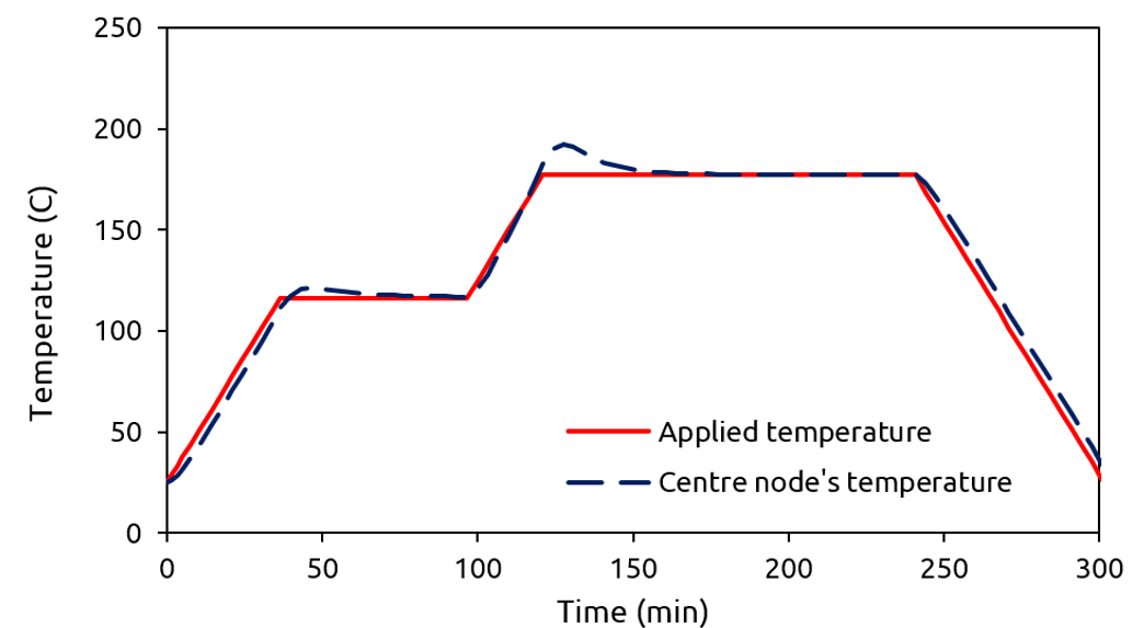
Figure 9: Comparison of the applied temperature and the temperature developed in a composite during curing
For a deeper understanding of composite curing simulation, you can explore our learning package “Curing process simulation in Abaqus“. It presents the formulations for calculating the internal heat during curing, with a specific focus on the well-known AS4/3501-6 prepreg.
Evaluation of stress components during the composite curing simulation
Stress prediction is a challenge for the numerical simulation of the composite curing process. This challenge arises due to the changes in the resin’s modulus of elasticity. It makes the composite curing simulation complex. As illustrated in Figure 10, the modulus starts very low and rises significantly during curing as chemical reactions take place. Finally, it reaches a constant value.
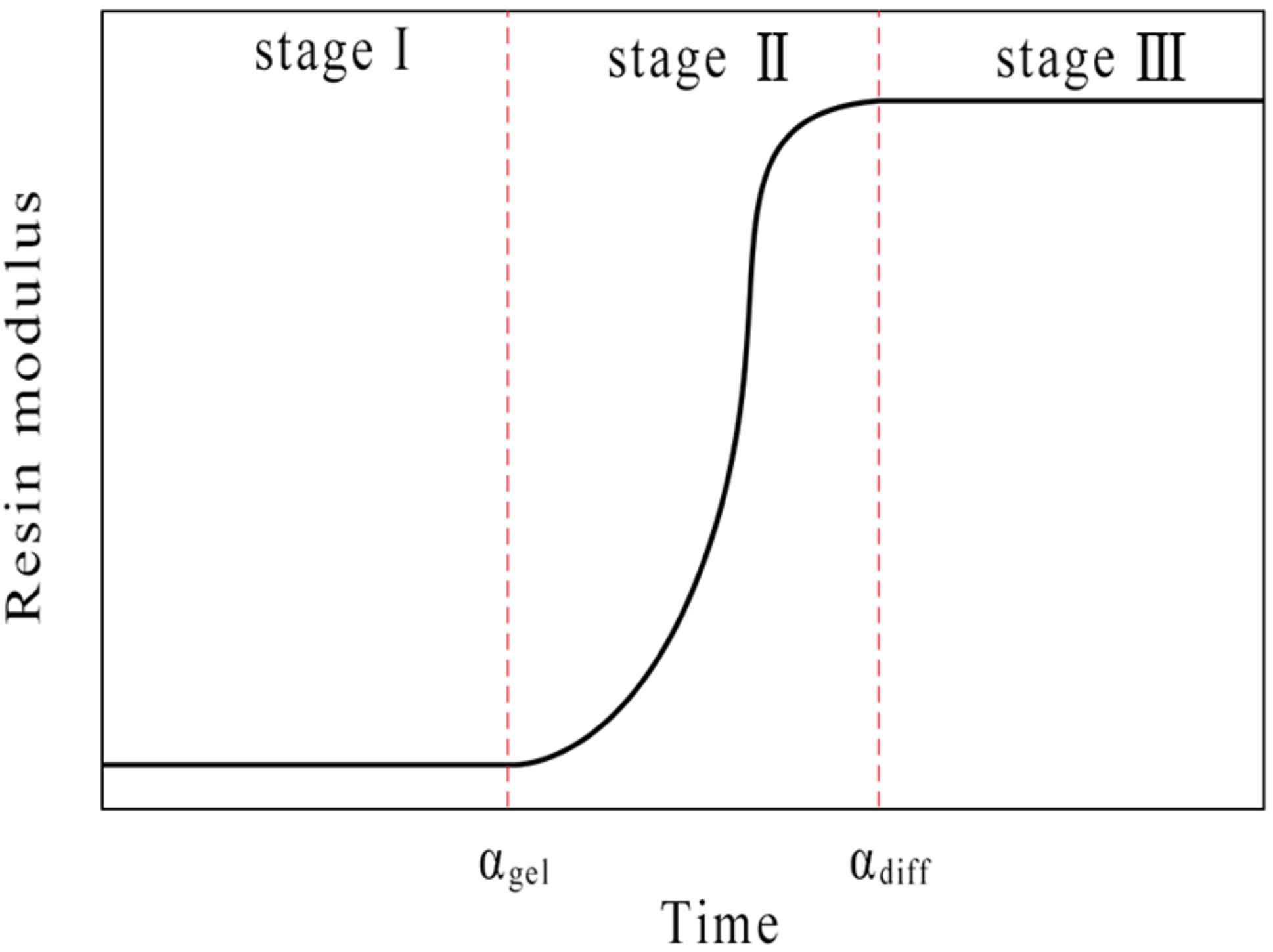
Figure 10: Schematic representation of the resin modulus variation during the curing process [Ref.]
Several models have been proposed to capture the variation of the resin’s modulus during composite curing simulation. The proposed models include linear-elastic, viscoelastic, and path-dependent ones. Each offers advantages and limitations. Table 1 summarizes the models specifically developed for calculating the resin modulus or stress components in the AS4/3501-6 prepreg. You can check this article “Effect of cure cycles on residual stresses in thick composites using multi-physics coupled analysis with multiple constitutive models” for more details on these models. They have simplified the composite curing simulation.
| Category | Model | Mathematical Formulation |
|---|---|---|
| Linear-elastic | Chile ($\alpha$) | $E_m = (1-\alpha)E_m^0 + \alpha E_m^{\infty}$ |
| Chile ($T$) | $E_m = \begin{cases} E_m^0 & T_* \le T_{c1} \\ \left( \frac{T_{c2}-T_*}{T_{c2}-T_{c1}} \right) E_m^0 + \left( \frac{T_*-T_{c1}}{T_{c2}-T_{c1}} \right) E_m^{\infty} & T_{c1} < T_* < T_{c2} \\ E_m^{\infty} & T_* \ge T_{c2} \end{cases}$ | |
| Viscoelastic | General Model | $\sigma_i(t) = \int_{0}^{t} C_{ij}(\xi-\xi’) \frac{\partial \epsilon_j}{\partial \xi’} d\xi’$ |
| Path-dependent | Temperature Dependent | $\sigma_i = \begin{cases} C_{ij}^0 \epsilon_j & T \ge T_g \\ C_{ij}^1 \epsilon_j – (C_{ij}^1 – C_{ij}^0) \epsilon_j |_{t=t_{vit}} & T < T_g \end{cases}$ |
In Table 1, the first two equations (Linear-elastic) models are used for curing simulation which you can learn the equations and how to model them completely in the Curing process simulation in Abaqus Tutorial.
Also, the next two equations (Viscoelastic & Path-dependent) models are used for curing simulation in the package below.
We have provided a detailed description of linear-elastic models and a step-by-step guide for their implementation within the provided package. It simplifies the composite curing simulation. For validation, we compared the results with reference solutions, as shown in Figure 21.
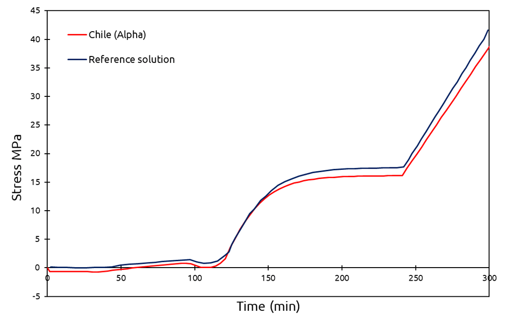
Figure 11: Comparison of the stress in a composite with the reference solution
In summary, numerical composite curing simulation requires the simultaneous consideration of thermal, chemical, and mechanical fields. You might be wondering how to implement such a complex model, but don’t worry! We will guide you through an accurate and efficient method to tackle this challenge.
Strain evaluation in FRCs during curing
The curing process can result in undesirable deformations in composites, and negatively impact product quality. To minimize these deformations, we should consider the residual strains in a fiber reinforced composite curing simulation.
During the curing process, composites experience two types of strain: mechanical and non-mechanical. The non-mechanical strains in composites originate from both cure shrinkage and thermal expansion. Cure shrinkage arises due to the release of gases and solvents, in the matrix, during the curing process. We can calculate it from the following equation.
$$\varepsilon_{cu} = \mathbf{CCS} \, \Delta \alpha$$
In this equation, CCS represents the effective chemical shrinkage coefficient of the matrix, and ∆α is the variation in the degree of cure. Figure 12 schematically illustrates how the chemical shrinkage occurs during the curing process.
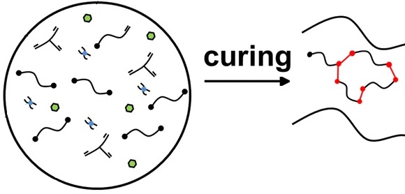
Figure 12: Illustration of the chemical shrinkage effect during the curing process (Adapted form [Ref.] with modifications)
The thermal expansion depends on both the externally applied heat and the internal heat generated during curing. Since the internal heat depends on the degree of cure, the thermal expansion is also influenced by the chemical reactions. You can calculate it from the following equation.
$$\varepsilon_{th} = \boldsymbol{CTE} \, \Delta T$$
Where CTE is the thermal expansion coefficient of the composite, and is the variation in its temperature.
In summary, several factors influence the total strain experienced by composites during curing, as detailed in Figure 13.
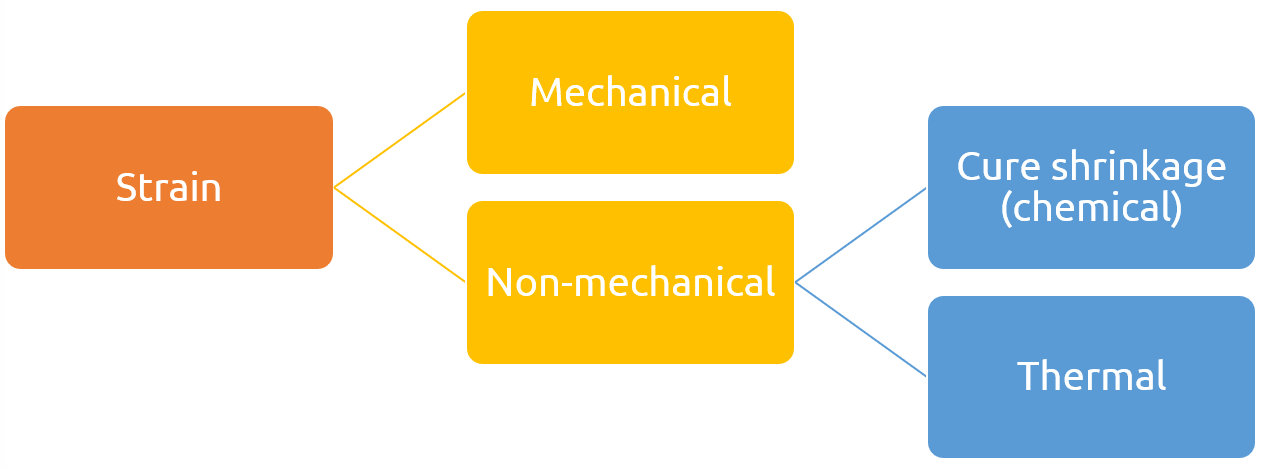
Figure 13: An overview of the strain components generated in a composite during the curing process
Considering all strain components together in a fiber reinforced composite curing simulation can be challenging. However, the “Curing process simulation in Abaqus” learning package on our website simplifies this process. It offers a step-by-step guide on calculating strain components during composite curing simulation. For validation, we compared our results with a reference solution, as shown in Figure 14.
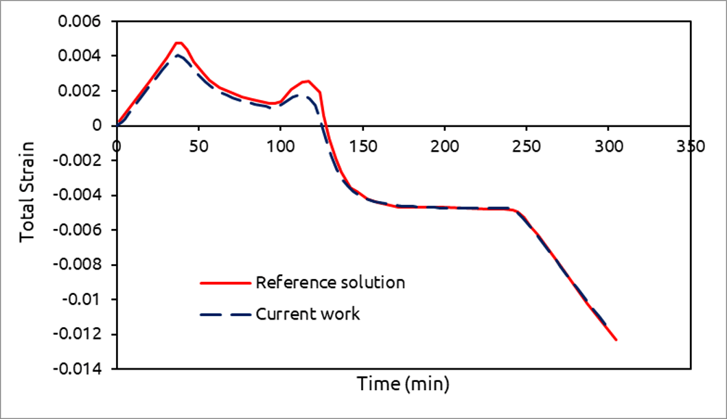
Figure 14: Comparison of the total strain in the composite with the reference solution
Abaqus curing process simulation
Abaqus is a widely used finite element program, that has simplified the fiber reinforced composite curing simulation.

It has been extensively used in published papers to analyze internal heat generation and mechanical fields during the composite curing process. However, the lack of required thermo-chemo-mechanical models in Abaqus presents a significant challenge for Abaqus curing process simulation.

Fortunately, Abaqus user-defined subroutines provide a powerful solution to overcome this challenge.
Composite curing simulation using subroutines
Have you ever heard of composite curing simulation using subroutines? Abaqus has a large number of user-defined subroutines with diverse functionalities. You need to utilize several subroutines simultaneously for the Abaqus curing process simulation.

Abaqus User Subroutines for Curing Process Analysis
| Subroutine | Purpose | Key Inputs | Outputs | Application |
|---|---|---|---|---|
| USDFLD | Define user field variables |
|
|
Calculates α and stores it for use in other subroutines. |
| UEXPAN | Calculate non-mechanical strains |
|
|
Calculates deformations caused by chemical reactions and temperature changes. |
| UMAT | Define custom mechanical behavior |
|
|
Calculates α-dependent mechanical properties and returns stresses to Abaqus. |
| HETVAL | Calculate internal heat generation |
|
Heat generation | Calculates exothermic heat from the curing reaction and passes it to the thermal solver. |
| DISP | Define complex boundary conditions |
|
Prescribed Boundary Conditions | Simulates complex thermal cycles and controls mold deformation. |
USDFLD subroutine
USDFLD is a subroutine that enables us to define user-defined field variables in Abaqus. You can use USDFLD to calculate the degree of cure and its variation with respect to time, for the composite curing simulation. The subroutine enables us to save these parameters as solution-dependent variables (SDVs). These SDVs can be called by other subroutines to calculate internal heat, non-mechanical strains, and stress components. The subroutine’s interface is shown in Figure 16.
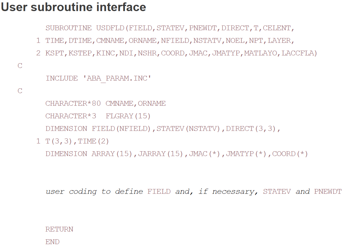
Figure 16: The user interface for the USDFLD subroutine
For further details on the USDFLD subroutine, you can refer to the learning package “Introduction to USDFLD and VUSDFLD Subroutine“ on our website.
UEXPAN subroutine
UEXPAN is another Abaqus subroutine that enables us to calculate non-mechanical strains during the composite curing process. The subroutine’s interface is presented in Figure 17.
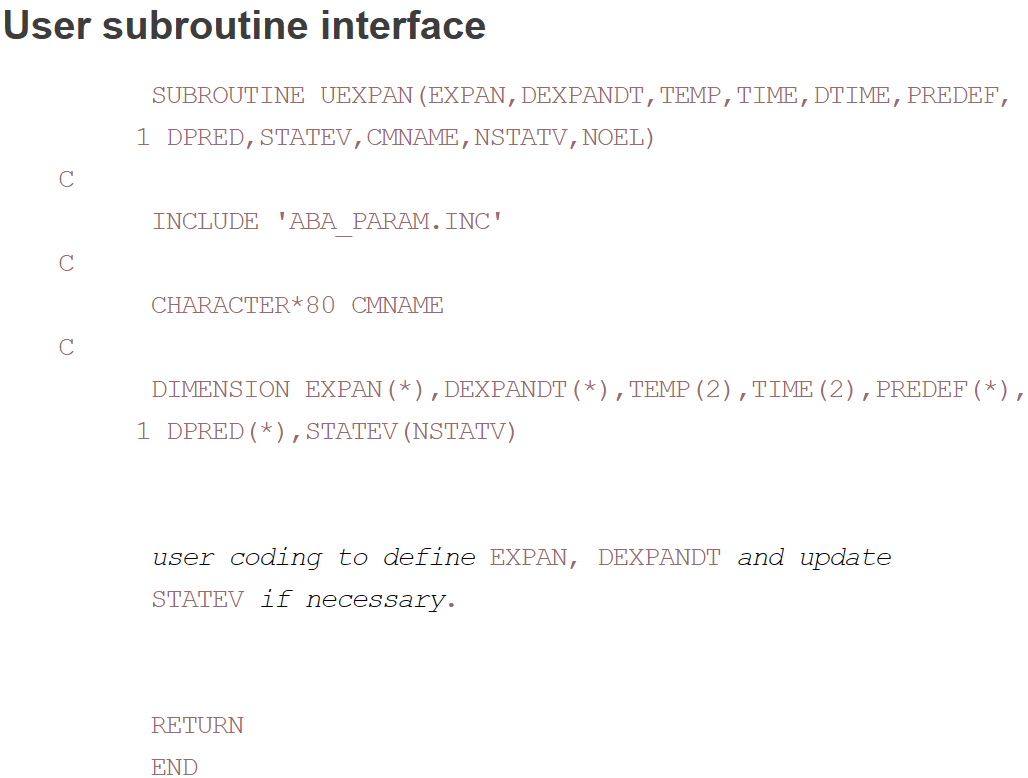
Figure 17: The user interface for the UEXPAN subroutine
Within UEXPAN, you can call state variables like the degree of cure to calculate cure shrinkage strains. Moreover, you can obtain the current temperature to calculate thermal expansion. For a detailed explanation of this subroutine, refer to the learning package “UEXPAN and VUEXPAN Subroutine” on our website.
UMAT subroutine
UMAT is a subroutine that allows users to define their desired material properties, particularly for models not available in the Abaqus library. It enables us to calculate the resin’s density as a function of the degree of cure, for the composite curing simulation. UMAT ultimately returns the calculated stress components to Abaqus for further calculations. The subroutine’s interface is shown in Figure 18.
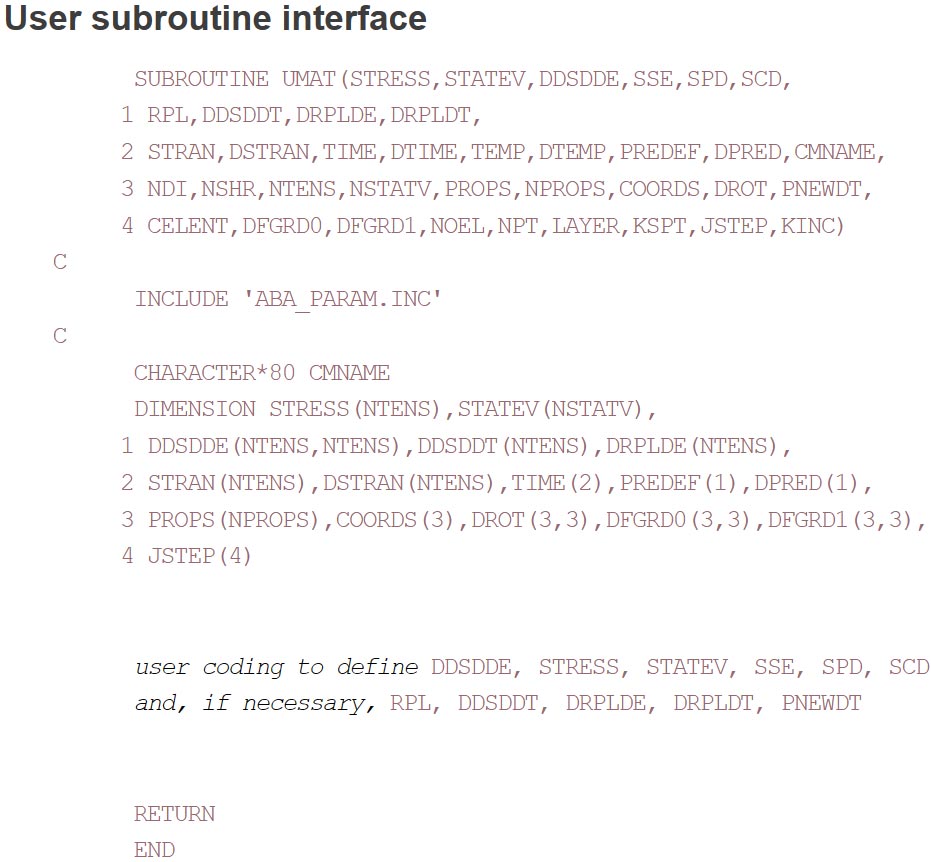
Figure 18: The user interface for the UMAT subroutine
For a basic introduction to writing UMAT subroutines, refer to this free tutorial “UMAT subroutine free tutorial“. Additionally, a more detailed tutorial with a step-by-step guide is offered for those interested in advanced applications in “UMAT subroutine introduction“.
HETVAL subroutine
HETVAL, another Abaqus subroutine, allows for calculating internal heat generation during the composite curing process. It enables the user to define the thermo-chemical model and calculate the heat generated due to chemical reactions. The subroutine retrieves the degree of cure and its derivative with respect to time from user-defined state variables, for the composite curing simulation. With this information, the subroutine calculates the internal heat and transfers it to Abaqus CAE for the solution process. The subroutine’s interface is shown in Figure 19.
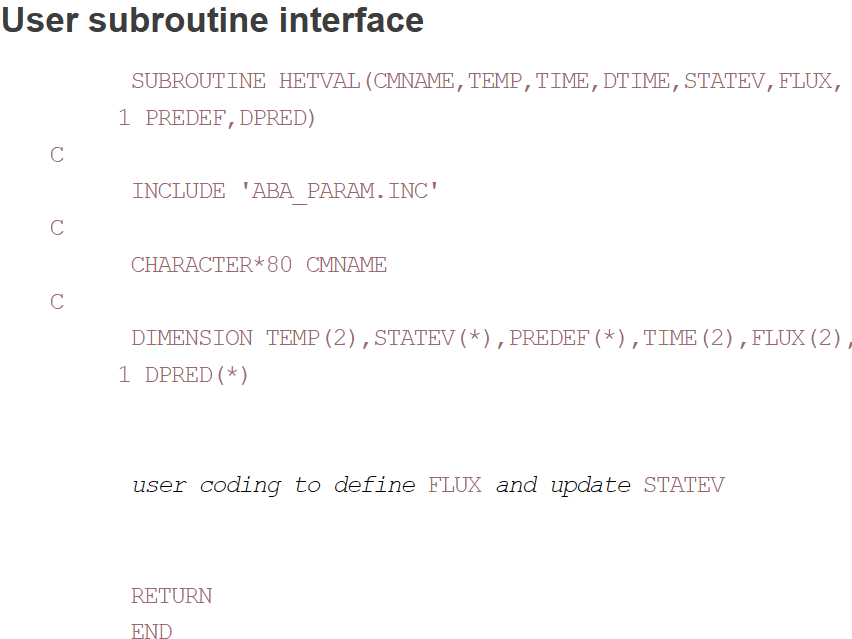
Figure 19: The user interface for the HETVAL subroutine
We recommend checking out this tutorial “HETVAL subroutine in Abaqus” on our website which shows how to write the HETVAL subroutine for different scenarios.
DISP subroutine
DISP is a subroutine that allows you to define complex boundary conditions. While Abaqus offers built-in features for defining boundary conditions for composite curing simulation, DISP provides more flexibility and control. So, the subroutine is useful for simulating the curing process under complex temperature cycles. Figure 20 presents the subroutine’s interface.
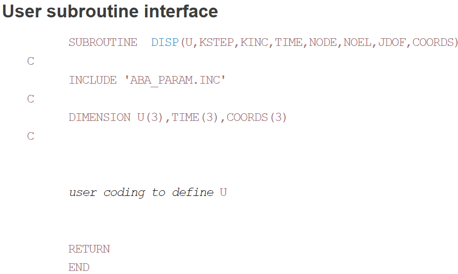
Figure 20: The user interface for the DISP subroutine
For more information on this subroutine, we recommend checking the provided learning package “DISP and VDISP subroutines in Abaqus“.
A learning package for the simulation of the curing process in Abaqus
Utilizing the mentioned subroutines to simulate the curing process is challenging, especially for those unfamiliar with the Fortran programming language. Moreover, defining the complex thermo-chemo-mechanical equations within the subroutines increases this difficulty. However, we have simplified the learning experience to help you overcome these challenges.
In the provided learning package “Composite Curing simulation“, you can gain a comprehensive understanding of the basics of fiber reinforced composite curing simulation using subroutines. Additionally, it helps you become familiar with a well-known thermo-chemo-mechanical model for fiber reinforced composite curing simulation in AS4/3501-6 prepreg. The tutorial provides a step-by-step guide for you to write all the mentioned subroutines and the Abaqus curing process simulation. For validation, we have compared the results of the composite curing simulation with those from the following papers. They have discussed the numerical modeling of the composite curing process in detail.
- Numerical Simulation and Multi-objective Optimization for Curing Process of Thermosetting Prepreg
- Effect of cure cycles on residual stresses in thick composites using multi-physics coupled analysis with multiple constitutive models
Abaqus version 2022 was used for the simulation. However, the procedure can also be applied to other versions, although there may be minor differences in some of them. For example, we also performed the simulation once in Abaqus 2024, and as shown in the figure below, we had to change the element type to hybrid; you can do the same as well.

For validation, several results such as the stress–time curve, strain–time curve, and the Deborah number were checked. You can see the details in the figure below. In this way, you can trust the results of the Abaqus simulation.


Summary
This article focused on the simulation of the composite curing process in Abaqus, particularly for fiber-reinforced composites (FRCs). The importance of understanding and optimizing this process lies in its direct impact on the quality, strength, and durability of composite materials, which are critical for applications in aerospace, automotive, and other high-performance industries.
The article began by discussing the nature of FRCs, their types, and the methods used to produce them. It then highlighted the advantages of FRCs over traditional materials and their broad applications. The article outlined the curing process, comparing oven-curing and autoclave methods, and emphasized the need for accurate simulations to optimize this process. The complexity of composite curing simulation was explored, detailing the thermo-chemo-mechanical aspects that need to be addressed. Finally, the article discussed the use of Abaqus subroutines to perform these simulations, specifically USDFLD, UEXPAN, UMAT, HETVAL, and DISP, which allow for detailed control and modeling of the curing process.
In conclusion, this article provided a comprehensive guide on simulating the composite curing process using Abaqus, covering essential methods, challenges, and tools required for accurate and efficient simulation. Through the use of specific subroutines, the article demonstrated how to achieve precise control over the curing process, ensuring the production of high-quality composites.
The CAE Assistant is committed to addressing all your CAE needs, and your feedback greatly assists us in achieving this goal. If you have any questions or encounter complications, please feel free to share it with us through our social media accounts including WhatsApp.
If you need deep training, our Abaqus Course offerings have you covered. Visit our Abaqus course today to find the perfect course for your needs and take your Abaqus knowledge to the next level!
You can always learn more about Abaqus in Abaqus Documentation.
Composite Curing FAQs
Basically, curing is when you apply heat and pressure to the composite so the resin hardens and turns from a liquid into a solid, giving the material its final strength.
Oven curing is simpler and cheaper, but the quality isn’t as high. Autoclaves, on the other hand, use both heat and pressure, so you end up with much stronger and cleaner parts.
Thermosets are kind of a one-way process—once they’re cured, that’s it, you can’t melt them again. But thermoplastics can be reheated and reshaped, which makes them more flexible in that sense.
Because curing isn’t just about heat—it’s a mix of chemical reactions, temperature changes, and mechanical effects all happening together. You need this type of simulation to really understand and predict what’s going on.
Residual stresses mainly come from the resin shrinking and the different thermal behavior between fibers and matrix as the part cools down.
It basically tells you how far the resin has gone in the curing process, and that directly affects the final properties, heat generation, and internal stresses.