
Predicting how materials respond under extreme conditions like high strain rates and elevated temperatures is crucial in various fields, like aerospace, automotive engineering, etc. The Abaqus Johnson-Cook model is a versatile and widely used constitutive model in the finite element analysis software Abaqus, which offers valuable insights into the dynamic response of materials under such demanding scenarios.
The Johnson-Cook model is a phenomenological material model, meaning it relies on experimental data to define the material’s response. This model captures the effects of strain rate, temperature, and strain hardening on the yield stress of a given material. It is particularly well-suited for simulating high-velocity impact, explosive loading, and other dynamic events where these factors play a crucial role.
In this article, we are going to discuss the Abaqus Johson-Cook model which involves Johnson-Cook plasticity and Johnson-Cook damage. We introduce each model and its dependent variables; So, you will understand how to improve your simulations using these models in Abaqus. Let’s Start.
Johnson–Cook Material Model – Video Explanation
Podcast: High-Velocity Impact & Johnson–Cook
| Model Name | Type | Key Parameters | Phenomena Captured | Primary Applications | Typical Materials |
|---|---|---|---|---|---|
| Johnson-Cook (JC) | Empirical / Viscoplastic | A, B, n, C, m, D1–D5 | Strain hardening, strain-rate sensitivity, thermal softening, ductile damage | Impact, penetration, crash, machining, explosive loading | Steel, copper, tantalum, aluminum alloys |
| Zerilli-Armstrong (ZA) | Physical / Dislocation-based | C0–C5 (or σa, B, β, B0, α, n) | Dislocation mechanics, grain size effects, thermal activation | High-rate structural dynamics | FCC & BCC metals |
| Mechanical Threshold Stress (MTS) | Physical / Dislocation-based | σa, σi, σe, g0, b, kB, θ0 | Microstructural evolution, intrinsic barriers | High-fidelity plasticity modeling | Copper, steel, aluminum alloys |
| Preston-Tonks-Wallace (PTW) | Physical / Viscoplastic | s0, s∞, y0, y∞, K, γ, θ, d | Extreme strain-rate deformation up to melt | Shock and hypervelocity impact | Metals under explosive loading |
| Steinberg-Cochran-Guinan-Lund (SCGL) | Semi-empirical / Viscoplastic | σa, β, n, σp, UK, C1, C2 | Pressure-dependent shear modulus | Shock physics | Metals, BCC materials |
| Cowper-Symonds | Empirical / Viscoplastic | C, P | Rate-dependent yield stress scaling | Crashworthiness analysis | Steel, aluminum alloys |
| Bingham-Norton | Elastic–Perfectly Viscoplastic | E, η, σy, λ, N | Yield followed by viscous flow | Yield-stress materials | Geomaterials, metals |
| Norton-Hoff | Perfectly Viscoplastic | λ, N (or K, m) | Secondary creep | High-temperature forming | Metals, polymers, asphalt |
Theoretical Background: Viscoplasticity
The Johnson-Cook model belongs to the theory of viscoplasticity. This theory explains how materials undergo permanent deformation based on the loading rate. Engineers often visualize this behavior using rheological models. For example, they use spring elements for elasticity and dashpots for rate dependence. While the JC model is purely empirical, it remains the most popular choice in engineering.
It effectively combines strain hardening, strain rate effects, and thermal softening into one simple, usable form.
Abaqus Johnson-Cook Model
The Johnson Cook (JC) material model is a constitutive model used to describe the behavior of metals under high strain rates and high-temperature conditions. It is widely used in finite element analysis (FEA) software, including Abaqus. The Johnson Cook model, developed by Johnson and Cook in 1983, proves to be a versatile tool for capturing the complex material response in situations like impact, penetration, and explosive forming.
The Abaqus Johnson Cook model as said before, involves two main sections:
- Johnson-Cook Plasticity
This section aims to define the hardening behavior of the material. Johnson Cook considers several factors such as plastic strain, strain rate, and temperature to define the material hardening in the plastic region.
- Johnson Cook Damage
The Johnson-Cook plasticity model can be used in conjunction with the progressive damage and failure models. One of the ductile damage models provided in Abaqus is the Johnson-Cook damage. This model is referred to as the “Johnson Cook dynamic failure model.
We start our discussion with the Johnson-Cook Plasticity. But before we start, if you are looking for a full tutorial with practical examples, I recommend visit this link which contains 4 Practical examples such as Drilling and Impact analysis.

Johnson Cook Plasticity
Johnson Cook plasticity is a constitutive material model used to describe the plastic behavior of metals under dynamic loading conditions, such as those encountered in high-speed machining, impact, and blast loading. It is a phenomenological model that incorporates strain, strain rate, and temperature effects on the material’s yield strength and flow stress.
A Mises yield surface with associated flow is used in the Johnson-Cook plasticity model. The Johnson-Cook hardening can be determined in two ways: one way is that the material yield stress is dependent on the plastic strain and the temperature. The second one not only defines the yield stress as a function of plastic strain and temperature but also adds the strain rate as the third factor to the formulation. First, we talk about the normal hardening, and then will talk about the rate-dependent one.
Johnson-Cook hardening
Johnson-Cook hardening is a particular type of isotropic hardening where the static yield stress,  , is assumed to be of the form:

where  is the equivalent plastic strain and A, B, n, and m are material parameters measured at or below the transition temperature,
 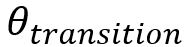 . The transition temperature is defined as the one at or below which there is no temperature dependence of the yield stress. Sometimes the room temperature is used in the formulations instead of the transition temperature.
 is the nondimensional temperature defined as:
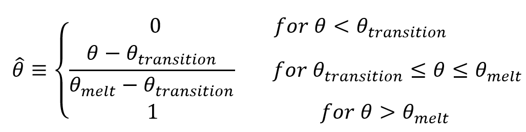
where  is the current temperature and
  is the melting temperature.
When 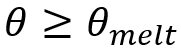 , the material will be melted and will behave like a fluid; there will be no shear resistance since
 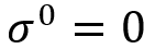 . The hardening memory will be removed by setting the equivalent plastic strain to zero.
In order to define this hardening for your analysis, you must provide the values of A, B, n, m, , and as part of the metal plasticity material definition.
In Abaqus/CAE to define this hardening type you must do as following:
- Go to the “Property” module
- Define a Material
- Mechanical Plasticity Plastic: Hardening: Johnson-Cook
The related window is shown in figure 1.
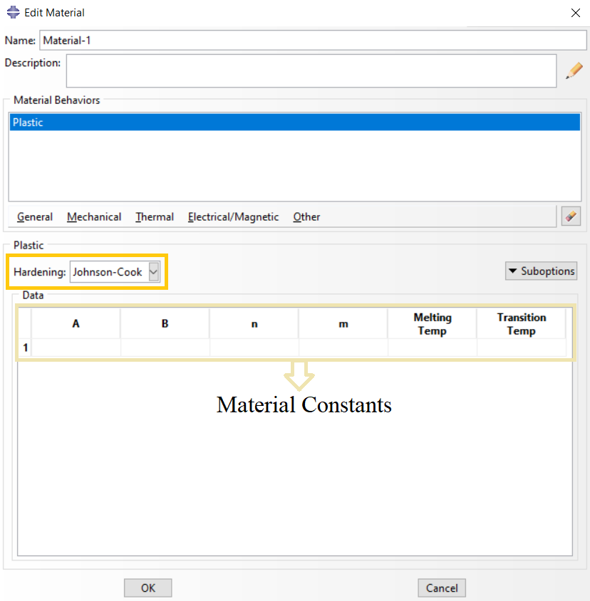
Figure 1: Defining Johnson-Cook hardening in Abaqus/CAE
Johnson Cook model strain rate dependence
Johnson Cook model strain rate dependence assumes that:

where  is the yield stress at nonzero strain rate;
  is the equivalent plastic strain rate;
 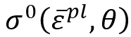 is the static yield stress; and
 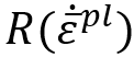 is the ratio of the yield stress at nonzero strain rate to the static yield stress.
The equivalent plastic strain rate can be calculated as:

 and C are material parameters measured at or below the transition temperature. (So that
 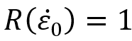 ).
).
Therefore, the Johnson-Cook strain rate-dependent yield stress is expressed as:

In addition to previous material constants, here you need to provide the values of C and when you define Johnson-Cook rate dependence.
In figure 2 the constants of the Johnson-Cook rate dependence model for some materials are listed. The value of 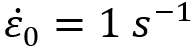 and is considered as the room temperature.
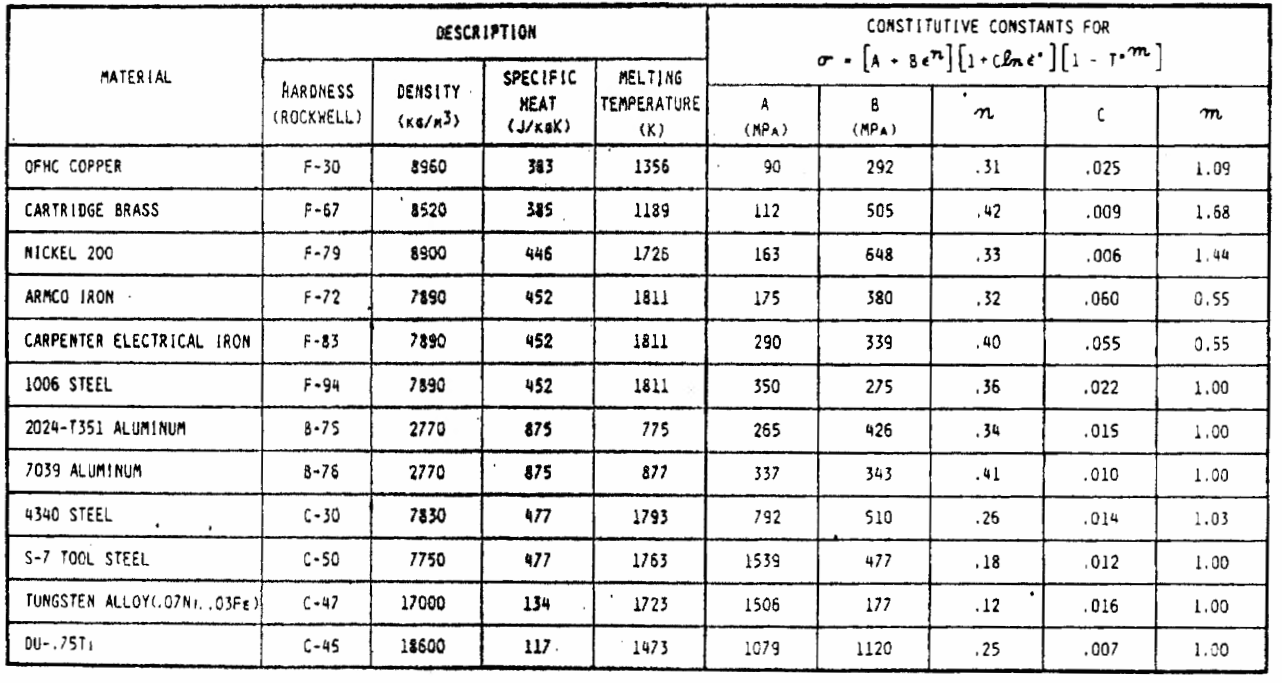
Figure 2: Constitutive constants for the various materials [1]
In Abaqus/CAE to define this hardening type you must do as following:
- Go to the “Property” module
- Define a Material
- Mechanical Plasticity Plastic: Hardening: Johnson-Cook: Suboptions Rate Dependent: Hardening: Johnson-Cook
The related window is shown in figure 3.
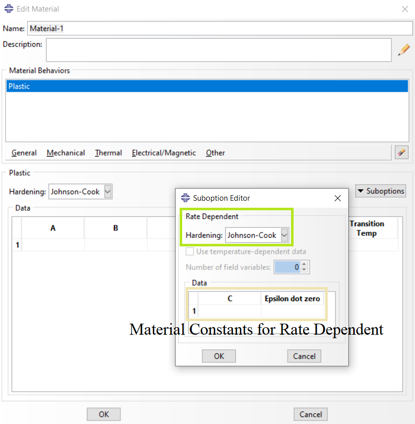
Figure 3: Defining Johnson-Cook Rate Dependent hardening in Abaqus/CAE
By now, we have reviewed the Johnson-Cook plasticity which includes two sections. Take a rest and when you are ready, we continue our discussion on Johnson-Cook damage. Here is an example of Johnson-cook plasticity: “Drilling simulation”
How to Calibrate and Validate JC Parameters
You must obtain accurate material constants for a reliable simulation. Typically, researchers use smooth round bar tensile tests to collect raw stress-strain data. Afterward, you can fit these curves using Excel or specialized software like CurveFitter.
First, identify the hardening parameters A, B, and n at a reference strain rate. Then, determine the strain rate coefficient C and thermal exponent m by varying test conditions. Furthermore, always validate these parameters before performing complex simulations. You should create a single-element model in Abaqus to replicate the physical test. This crucial step confirms that your input data produces the expected results. Additionally, consider applying strain rate filtering during dynamic analyses. This technique damps non-physical vibrations and provides smoother, more realistic output.
Johnson-Cook Damage
The Johnson-Cook damage model is a constitutive model used to describe the ductile failure of metals under dynamic loading conditions. It is a phenomenological model that incorporates strain, strain rate, and temperature effects on material damage.
Abaqus/Explicit provides a dynamic failure model specifically for the Johnson-Cook plasticity model, which is suitable only for high-strain-rate deformation of metals. This model is referred to as the “Johnson-Cook dynamic failure model”.
Abaqus/Explicit also offers a more general implementation of the Johnson-Cook failure model as part of the family of damage initiation criteria, which is the recommended technique for modeling progressive damage and failure of materials. To get more familiar with damage, especially in ductile materials, we recommend seeing the following article as well:
“Ductile Damage: A Comprehensive Study on Failure Mechanisms of Ductile Materials”
Johnson-Cook dynamic failure model
The Johnson-Cook dynamic failure model is based on the value of the equivalent plastic strain at element integration points. Failure is assumed to occur when the damage parameter exceeds 1. The damage parameter,  , is defined as:
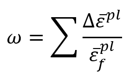
where  is an increment of the equivalent plastic strain,
  is the strain at failure, and the summation is performed over all increments in the analysis.
The strain at failure, , is assumed to be dependent on a nondimensional plastic strain rate,  ; a dimensionless pressure-deviatoric stress ratio,
  (where p is the pressure stress and q is the Mises stress); and the nondimensional temperature, , defined earlier in the Johnson-Cook hardening model. The dependencies are assumed to be separable and are of the form:

Where  to
to  are failure parameters measured at or below the transition temperature, , and
  is the reference strain rate.
[/vc_column_text][/vc_column][/vc_row]
To define the Johnson-Cook dynamic failure model, you must provide the values of to . Similar to the Johnson-Cook hardening, you also need to determine the values of the transition temperature, , melting temperature, , and reference strain rate, . The values of these constants are shown for three materials in figure 4. Note that most materials experience an increase in with increasing pressure-deviatoric stress ratio; therefore,  in the above expression will usually take positive values in contrast to figure 4 values for .
When this failure criterion is met, the deviatoric stress components are set to zero and remain zero for the rest of the analysis. By default, the elements that meet the failure criterion are deleted.
The Johnson-Cook dynamic failure model is suitable for high-strain-rate deformation of metals; therefore, it is most applicable to truly dynamic situations.
The use of the Johnson-Cook dynamic failure model requires the use of Johnson-Cook hardening but does not necessarily require the use of Johnson-Cook strain rate dependence. However, the rate-dependent term in the Johnson-Cook dynamic failure criterion will be included only if the Johnson-Cook strain rate dependence is defined.
Johnson-Cook dynamic failure is not supported in Abaqus/CAE.
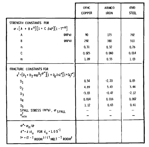
Figure 4: Strength and Fracture constants for three materials ( is the stress triaxiality) [2]
Johnson-Cook damage initiation criterion
The material damage initiation capability for ductile metals is intended as a general capability for predicting the initiation of damage in metals.
The Johnson-Cook criterion (available only in Abaqus/Explicit) is a special case of the ductile criterion in which the equivalent plastic strain at the onset of damage,  , is assumed to be of the form:

Most of the materials experience a decrease in with increasing stress triaxiality 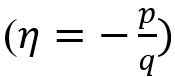 ; therefore, in the above expression will usually take positive values.
You can use the following option to specify the parameters for the Johnson-Cook initiation criterion:
- Go to the “Property” module
- Define a Material
- Mechanical Damage for Ductile Metals Johnson-Cook Damage
The related window is shown in figure 5.
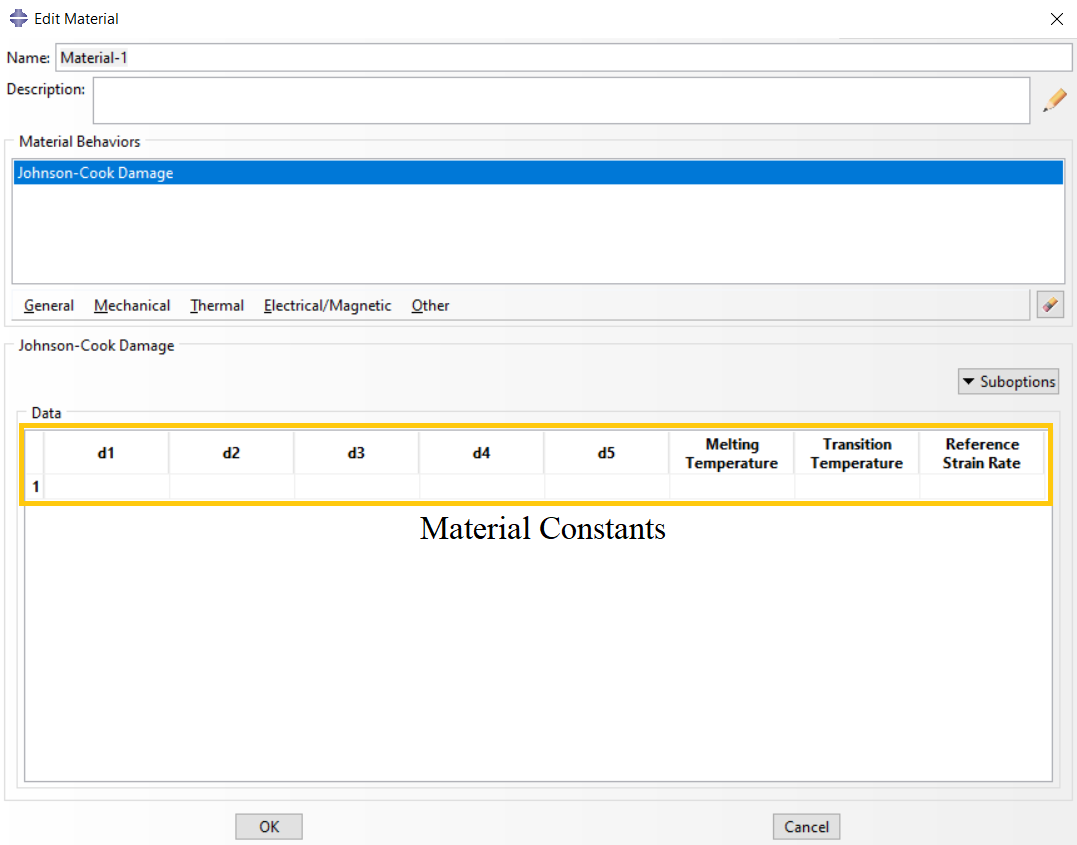
Figure 5: Defining Johnson-Cook damage initiation in Abaqus/CAE
Here is the end of this section. Let’s summarize what we have learned in this article. Here is an example of Johnson-Cook damage: “Johnson-cook plasticity and damage initiation”
Summary
We started with the definition of the Johnson-Cook model. Johnson-Cook model consists of two sections: Plasticity and Damage. We have reviewed both sections to give you an insight into them in case of implementation in your analyses. In conclusion, we can mention the Johnson-Cook model’s advantages and limitations as follows:
Advantages
- It is relatively simple to implement and calibrate.
- It accounts for the effects of strain, strain rate, and temperature.
- It can accurately predict the failure of materials under a wide range of loading conditions.
Limitations
- It is a phenomenological model and may not provide a fundamental understanding of the material’s behavior.
- It may not be accurate for all materials or loading conditions.
- It requires extensive experimental testing to determine the material parameters.
The Johnson-Cook model is a valuable tool for simulating high-strain-rate deformation in Abaqus. It provides a relatively simple yet accurate representation of material behavior under challenging conditions. By understanding the model’s strengths and limitations, engineers can use it effectively for various applications, including impact analysis, penetration mechanics, and explosive forming.
To get more familiar with the Abaqus Johnson-Cook model, you can see the following link which has several workshops using Johnson-Cook plasticity and damage models in simulations:
Explore our comprehensive Abaqus tutorial page, featuring free PDF guides and detailed videos for all skill levels. Discover both free and premium packages, along with essential information to master Abaqus efficiently. Start your journey with our Abaqus tutorial now!





 English
  Korean
  Chinese
One Response
I was struggling with setting up the JC damage parameters for a drilling simulation, and your explanation of the material constants was exactly what I needed. The inclusion of ready-to-run .inp examples and the VUMAT training makes this resource much more practical than a standard textbook.