
Creep is the slow, time-dependent deformation of solid materials. This permanent strain happens under constant load, even when the stresses are well below the material’s yield strength.
Understanding and accounting for creep behavior is vital for designing reliable components. This phenomenon is critical in high-temperature structures, such as pressure vessels, boiler tubes, turbine blades, and jet engines. Therefore, engineers must utilize creep simulation to predict long-term structural reliability and prevent catastrophic failure cheaply and efficiently.
This guide provides the necessary theoretical foundation (creep in materials) and delivers essential, expert guidance for accurate Abaqus creep simulation.
Creep is the slow, permanent deformation of a solid material. It occurs when the material is subjected to a constant load and elevated temperature over a long time.
Abaqus handles creep by dividing the analysis into two sequential steps: Static (to establish initial stress) and Visco (to simulate time-dependent deformation). Parameters needed include elastic properties, plus creep constants (A,n,m,Q).
Yes, alloying elements like aluminum and titanium, combined with nickel, are essential for forming precipitates (like in superalloys). These precipitates act as barriers that severely impede the movement of dislocations, which are the atomic-level carriers of creep strain.
Creep is a problem if the operating temperature exceeds the material’s critical homologous temperature (typically 0.4Tm) and if the predicted life falls below the design life, as determined using lifetime prediction tools like the Larson-Miller Parameter.
Their fundamental structures dictate their creep behavior. Metals creep due to dislocation and diffusion mechanisms at high temperatures (>0.4Tm). Polymers creep at much lower temperatures due to molecular chain movement (viscoelasticity). Ceramics typically resist creep strongly due to high melting points but deform via diffusion creep mechanisms.
What is Creep in materials? Three Stages of Creep
Creep is the slow, permanent deformation of a solid material. It occurs when the material is subjected to a constant load and elevated temperature over a long time.
Creep is a time-dependent inelastic deformation. It occurs even when the applied stresses are significantly below the material’s elastic limit or yield stress. This deformation is permanent because it results from changes to the material’s inherent atomic or molecular structure. In practice, creep is extremely important for components like pressure vessels, jet engines, and turbine blades.
Creep deformation typically follows three sequential stages:
- Primary Creep (Transient Stage)
- Secondary Creep (Steady-State Stage)
- Tertiary Creep (Accelerating Failure)
Analyzing these stages helps engineers interpret material response over its lifetime.
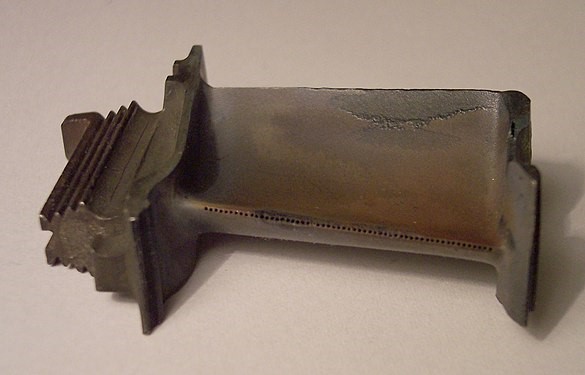
Figure 1: The turbine blade is damaged due to creep [Ref]
Three Stages of Creep in Materials
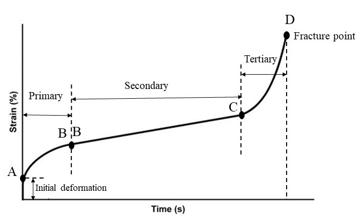
Typical creep curve showing the three stages: primary, secondary, and tertiary
Creep is generally considered an irreversible, inelastic process for metals. However, some materials like concrete and viscoelastic polymers exhibit partial recovery when the load is removed. For metals, creep is plastic deformation that lacks recoverability. Conversely, materials like concrete exhibit creep recovery when the load is removed, but this recovery is never complete. Polymers also show viscoelastic creep, characterized by both elastic (recoverable) and viscous (permanent) components.
Creep susceptibility depends on the homologous temperature (T/Tm), which is the ratio of operating temperature to the melting temperature. Most engineering metals require temperatures greater than 0.4Tm to creep. Creep is driven by thermally activated processes, such as atomic diffusion. For most metals, the energy barriers for atomic movement are only overcome at high temperatures, typically above half their melting point (0.5Tm). However, polymers and certain low-melting-point metals can experience significant creep closer to ambient conditions because they have much lower energy barriers for molecular rearrangement or diffusion.
Creep is primarily tested by applying a constant load or constant stress to a specimen at a specific, elevated temperature for a prolonged duration, often months or years. In a standard test, the specimen is loaded (creating instantaneous strain) and placed in a furnace to maintain a specific temperature (e.g., 50%Tm). The resulting elongation (strain) is then monitored over time. Testing uses two main methods: 1. Constant Load Method: The applied load stays constant, causing the stress to increase gradually as the cross-sectional area decreases during deformation. 2. Constant Stress Method: The applied force is adjusted dynamically to ensure the stress remains constant, even as the cross-sectional area changes. This method often eliminates the tertiary stage of creep on the curve.
Why Does Creep Occur in Materials? The Physics Behind Creep
Creep is fundamentally caused by the thermally activated motion of defects within the material’s structure. At elevated temperatures, these defects (primarily vacancies and dislocations) move and rearrange themselves, causing permanent strain under sustained stress.
Creep in materials is not merely a macroscopic failure; it is a complex, irreversible process driven by microstructural physics. When components operate at temperatures above their critical homologous temperature (typically 0.4Tm), sufficient thermal energy becomes available to activate atomic or microstructural processes. This energy allows crystalline defects to overcome local energy barriers.
The permanent deformation is therefore governed by three main categories of movement within the crystal lattice and grain structure:
- Dislocation Motion: The movement of line defects (dislocations) through the crystal lattice via climb and glide.
- Atomic Diffusion: The migration of atoms or vacancies through the lattice or along grain boundaries.
- Grain Boundary Sliding (GBS): The relative tangential motion of adjacent grains.
The dominant mechanism depends heavily on the specific stress and temperature conditions. Understanding which mechanism controls the deformation rate is the first step in performing a meaningful creep simulation.
Since multiple thermally activated processes drive this material degradation. The resulting creep in materials is rarely controlled by a single factor. Indeed, the macroscopic strain rate depends heavily on the specific interplay of applied stress, temperature, and microstructure (such as grain size). Therefore, to perform reliable creep simulation, engineers must rigorously define the fundamental kinetic laws that govern each dominant physical process. The following sections detail these essential mechanisms, including dislocation creep and diffusion creep, which dictate the material’s time-dependent response.
Diffusion-Controlled Creep (Low Stress/Nabarro-Herring and Coble)
Diffusion processes dominate the creep response at high temperatures and low stresses.
- Nabarro-Herring Creep (Lattice Diffusion):This mechanism involves atom diffusion through the crystalline lattice (bulk diffusion). The movement is driven by stress-induced vacancy gradients. Consequently, the creep strain rate scales inversely with the square of the grain size (
 ).
).
 ).
).
where  is the strain rate, σ is the applied stress, d is the grain size, Qd is the activation energy for diffusion, R is the universal gas constant, T is the absolute temperature, and A1 is a material-dependent constant.
- Coble Creep:This mechanism involves atomic transport concentrated along the grain boundaries. Coble creep dominates in fine-grained materials. Therefore, the strain rate scales inversely with the cube of the grain size (
 ).
).

Dislocation Creep (Power Law Creep/Norton’s Law)
Dislocation creep controls deformation at moderate to high stress levels. It is characterized by the movement of dislocations. Dislocations move via glide and thermally activated climb.
Climb allows dislocations to bypass obstacles by exchanging vacancies with the lattice. The steady-state strain rate follows the Norton Power Law, where the rate is proportional to the stress raised to a power n. For dislocation creep, the stress exponent typically ranges from 3 to 8.

The equation clearly demonstrates the exponential dependency on temperature (T) and the nonlinear dependency on stress ( ), where is the stress exponent.
Solute Drag Creep
Solute drag creep is a mechanism characterized by the resistance imposed by solute atoms on dislocation motion. Solute atoms cluster around the dislocation core, forming a Cottrell atmosphere. As a result, the dislocation requires a higher energy to break away from this cluster. This mechanism enhances creep resistance by increasing the effective activation energy required for dislocation movement.
Some most Common Questions of Creep Microstructural Mechanisms
Grain size has a complex and inverse effect on creep resistance, primarily depending on the dominant mechanism. The relationship changes drastically depending on whether lattice diffusion (Nabarro-Herring) or grain boundary diffusion (Coble) is controlling the rate.
Different diffusion mechanisms exhibit distinct grain size dependencies: Nabarro-Herring Creep (Lattice Diffusion): The creep strain rate is inversely proportional to the square of the grain size (∝d-2). Consequently, larger grains resist creep better in this regime. Coble Creep (Grain Boundary Diffusion): This mechanism dominates in fine-grained materials. The creep strain rate is inversely proportional to the cube of the grain size (∝d-3). Therefore, creep accelerates rapidly as grain size shrinks in this regime.
The accelerated deformation leading to rupture (tertiary creep) is primarily caused by microstructural damage. This damage includes the formation and growth of internal microscopic cavities (voids) and the subsequent development of microcracks.
- Void Nucleation and Growth: Microscopic voids nucleate at boundaries and inclusions, growing due to atomic diffusion and localized plastic deformation.
- Microcrack Formation: Voids coalesce (join together) to form microcracks, further accelerating failure.
- Grain Boundary Sliding: Increased sliding along grain boundaries exacerbates stress concentrations and damage.
- Necking and Localization: Macroscopic reduction in the cross-sectional area (necking) concentrates the stress, leading to localized deformation and eventual rupture.
Norton’s Law describes the constant strain rate during the secondary creep stage only. Time-Hardening and Strain-Hardening models are more complex viscoplastic frameworks that incorporate time or accumulated strain to capture the transient primary creep phase.
- Norton-Bailey Law: This simple power law (ϵ˙cr = A(T)σn) only models the steady-state (secondary) creep rate. It assumes strain rate depends only on stress and temperature.
- Time-Hardening Law: The creep rate depends explicitly on the elapsed time and stress (ϵ˙cr ∝ σn tm-1). Consequently, material resistance increases solely based on time, irrespective of the actual accumulated strain.
- Strain-Hardening Law: The creep rate depends on the accumulated creep strain (ϵ˙cr ∝ σn ϵcrp). This model is usually superior for situations where stress changes over time, as material resistance depends on its deformation history.
How Does Abaqus Handle Creep Simulation?
Abaqus handles creep by dividing the analysis into two sequential steps: Static (to establish initial stress) and Visco (to simulate time-dependent deformation). Parameters needed include elastic properties, plus creep constants (A,n,m,Q).
- FEA Step Setup:A creep analysis requires an initial Static step to evaluate the instantaneous stress state under applied loads. This stress state is then imported into the Visco step, which assesses the time-dependent creep behavior over the required long duration (e.g., 1,000 hours).
- Material Parameters:You must input standard elastic properties (Young’s Modulus and Poisson’s ratio). For creep, constants like the power law multiplier (A), stress exponent (n), time/strain exponent (m or p), and often the activation energy (Q) are required.
So far, numerous models have been developed for creep analysis, and Abaqus creep incorporates some of the best creep analysis models. In the following sections, we will introduce some of these models.
Time Hardening law
When the temperature or stress conditions vary during loading, hardening conditions should be considered. One of these conditions is hardening proportional to time. In this case, relations for creep strain variations over time can be obtained. One of the models provided by Abaqus creep for creep analysis is the time hardening law. This model accounts for hardening based on time and its relation is as follows:

Time Power law
The time-hardening model mentioned cannot accurately predict creep when stress changes. Additionally, using this method in Abaqus software sometimes faces computational problems. For these reasons, the time power law has been developed as an alternative to the time hardening law, which does not pose computational issues for Abaqus software. This model utilizes the following relation to predict creep:
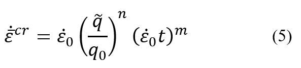
Strain Hardening law
Similar to the time hardening law, this model is also used when creep is accompanied by hardening. However, this model is particularly suitable for situations where stress changes over time and generally at low-stress levels. The relation for predicting creep according to this law is as follows:

Creep power law
creep analysis in Abaqus using the strain hardening law, such as the time hardening law, there are computational issues present in Abaqus, and sometimes Abaqus is unable to solve the creep problem using this model. For this reason, you can utilize the creep power law. This law, similar to the strain hardening law, can predict creep in situations where strain hardening relation exists due to stress changes. Moreover, there are no computational issues associated with using the creep power law. The creep power law is recognized as one of the best and most practical models for predicting creep. The following relation is used to predict creep using the creep power law:

Abaqus creep subroutine
Abaqus is a highly powerful finite element software, but sometimes users have needs that are not preconfigured in Abaqus. To address this issue, Abaqus recommends using subroutines. Users can fulfill their specific requirements by utilizing subroutines in a predetermined format.
Various models have been provided in the Abaqus for creep analysis, some of which we have reviewed in previous sections. Occasionally, Abaqus users may require the use of specialized or advanced models for creep analysis. For this category of users, Abaqus recommends using the Abaqus creep subroutine. Utilizing the Abaqus creep subroutine can also assist users in simulating complex creep analysis problems within Abaqus.
As you have already noticed, creep is a highly important phenomenon in engineering. Therefore, understanding this phenomenon, creep analysis, identifying its influential factors, and finding ways to predict and simulate it are of great significance. One way to predict creep in components with low cost is through creep analysis in Abaqus. However, as you know, this also comes with its own complexities.
You can learn how to write an Abaqus subroutine from the very beginning by simply read our free blog: How to Write Abaqus Subroutine?
For this reason, our team has decided to address all your needs in the form of a tutorial training package.
Do Cyclic Loads Accelerate Creep Compared to Steady Loading?
Yes, when loads are variable, the choice of hardening model becomes critical and affects the calculated creep rate. Under variable stress, the Time Hardening model and the Strain Hardening model will produce different results.
When stress is constant, both Time Hardening and Strain Hardening models yield identical creep strain results. However, if the traction varies over time (using an amplitude function), the two models diverge, demonstrating different material responses. This difference is crucial because variable loads can accelerate damage accumulation, impacting component life.
I’m Seeing Too Much Deformation Early in My Abaqus Creep Simulation—What Might Be Causing That?
Excessive early deformation is often caused by using poorly formulated or outdated creep models, especially those with explicit time dependence.
Engineers should avoid certain models that rely explicitly on time (like the Time Power Law, Model 8), as this can lead to “weird” or “goofy” responses. For example, a specimen sitting unloaded for a long time will behave differently when loaded, just because time has passed. Furthermore, older models like the Time Law and Strain Law should be avoided because better, better-formulated versions exist, such as the Creep Power Law (Strain-Dependent Model).
What Are the Pros and Cons of Using a User-Defined CREEP Subroutine?
Subroutines (e.g., Abaqus CREEP subroutine) allow engineers to implement complex, custom, or advanced creep models that are not available in the built-in library. However, they require expertise in coding (Fortran) and extensive validation.
Abaqus provides built-in models for standard creep analysis. Nonetheless, for users requiring specialized or advanced models, Abaqus recommends utilizing the user subroutine capability. Subroutines are necessary for solving complex creep analysis problems, such as those involving the Theta projection method for turbine blades.
Engineering for Longevity: Design and Life Prediction
The rigorous simulation of creep behavior is only one part of the engineering solution. Successful high-temperature design requires a dual focus to guarantee longevity and prevent structural failure. First, engineers must proactively improve the material’s innate resistance to creep in materials failure.
This involves sophisticated microstructural strategies designed to increase the activation energy required for permanent deformation. Second, reliability mandates accurately predicting the remaining service life. This step is necessary to set safe operational limits and prevent catastrophic rupture. Therefore, this section explores the critical strengthening mechanisms (Section 4.1) and the necessary empirical and mathematical tools for creep lifetime prediction (Section 4.2).
Strengthening Mechanisms
- Precipitation Strengthening:This method involves introducing fine, stable precipitates, such as the
 phase in nickel-based superalloys. These precipitates act as strong barriers to dislocation movement. Dislocations are often forced to bypass them through the Orowan looping mechanism. This bypass mechanism creates a threshold stress (
 ) that must be overcome. Consequently, the effective stress driving the creep is reduced, which significantly decreases the creep rate.
 - Solid Solution Strengthening:Solute atoms introduce lattice distortions that impede dislocation climb and glide. These solutes create a drag force on dislocations and reduce the effective diffusion coefficient by forming solute-vacancy complexes. This interaction effectively increases the activation energy required for the creep process.


Creep Lifetime Prediction
Engineers use empirical models to estimate the time required for failure (tr) under service conditions.
Generally, creep lifetime refers to the duration that a component can withstand creep before failure occurs. There are various models available for estimating creep lifetime, and we will examine some of the most well-known ones.
Larson Miller Estimation Model
This model estimates creep lifetime based on the Larson-Miller parameter. This parameter is derived from the creep rupture data and expresses a relation between temperature and the time required for creep rupture. Eq (1) expresses the time to creep rupture (tr) in terms of the Larson-Miller parameter (PLM), the Larson-Miller constant (CLM), and temperature (T).


Figure 6: Larson-Miller parameter values based on stress [Ref]
As mentioned, in this method, the Larson-Miller parameter is obtained using empirical data.
Orr-Sherby-Dorn Estimation Model
Similar to the Larson-Miller model, the Sherby-Dorn model estimates creep lifetime based on the Sherby-Dorn parameter. This parameter is also derived from empirical data. In the equation of this model, the time to creep rupture is expressed in terms of the Sherby-Dorn parameter (POSD), temperature (T), activation energy (Q), and the universal gas constant (R).

Polynomial Estimation Models
In creep analysis, there are models that estimate creep lifetime based on other models. These models are polynomial models. For example, the polynomial Larson-Miller model operates based on the Larson-Miller model. The difference in this approach is that instead of using empirical data to obtain the Larson-Miller parameter, a polynomial is used.
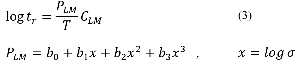
There are numerous methods for estimating creep lifetime that can assist us in creep analysis. However, these models, especially polynomial models, can also be used in creep analysis in Abaqus using the Abaqus creep subroutine, as they are based on theoretical relations.
Conclusion
Creep deformation is a major engineering challenge for materials operating under sustained stress and high temperatures. Accurate creep simulation requires integrating both the detailed physics of creep in materials (diffusion, dislocation movement, void growth) and the specific numerical requirements of the FEA solver.
Successful simulation depends on using appropriate modern models (like the Creep Power Law) and actively avoiding older or explicitly time-dependent laws due to inherent computational issues. Ultimately, material resistance is governed by microstructural design, focusing on creating obstacles (like precipitates or solute atoms) that increase the material’s activation energy and suppress the movement of dislocations.
Explore our comprehensive Abaqus tutorial page, featuring free PDF guides and detailed videos for all skill levels. Discover both free and premium packages, along with essential information to master Abaqus efficiently. Start your journey with our Abaqus tutorial now!






 English
  Korean
  Chinese