Under constant load, some materials keep deforming little by little, showing that stress is not just about force but also about time. They slowly change shape over time, depending not only on how much load is applied but also on how long it lasts. This time-dependent behavior is what makes them different from purely elastic or plastic materials.
This behavior is known as viscoplasticity, and it shows up in metals at high temperatures, polymers, soils, and even asphalt on the road. Unlike simple plasticity, viscoplasticity accounts for both the rate and duration of loading, which makes it important for engineers who need to predict how structures will behave in real-world conditions.
In this blog, we will first explain the basics of viscoplasticity and how it compares with other material models. Then, we’ll look at how Abaqus handles viscoplastic behavior through built-in options like rate-dependent plasticity, creep, and viscosity. Finally, we’ll cover the Perzyna viscoplastic model and show how it can be applied to load during time.
What is Viscoplasticity?
Viscoplasticity describes how certain materials respond to stress over time. It combines two fundamental behaviors: plasticity and viscosity.
Plasticity is the ability of a material to undergo permanent deformation once the applied stress exceeds a certain threshold, called the yield stress. Below this stress, the material behaves elastically and returns to its original shape. Beyond it, the deformation remains even after the load is removed.
Viscosity represents a material’s resistance to flow. A purely viscous material deforms gradually under an applied stress, and the rate of deformation depends on the stress magnitude. All deformation is permanent, and it continues as long as stress is applied.
When these two effects combine, the material exhibits viscoplastic behavior. This means deformation is both rate-dependent and time-dependent. The higher the stress, the faster the material flows (rate dependence), and the longer the stress is applied, the more it deforms over time (time dependence). Unlike purely plastic materials, which deform instantly once yielding starts, viscoplastic materials flow gradually, making both stress and duration important in their response.
Examples:
- Metals at high temperature, like turbine blades in jet engines, fail slowly under constant stress.
- Polymers and plastics under long-term loading (like a plastic chair sagging over the years).
- Soil and asphalt, which deform progressively under repeated traffic loads.

Figure 1: An example of viscoplastic loading that has led to a rupture in the pipe over time
To better understand viscoplasticity, it helps to compare it with other well-known models of material behavior. Each focuses on different aspects of time- or rate-dependent material behavior:
- Plasticity: These describe irreversible deformation once the yield stress is exceeded, but they are essentially rate-independent, unlike Viscoplasticity, which includes dependency.
- Viscous behavior: describes materials that deform continuously under stress. The rate of deformation depends on the magnitude of the stress and the duration it is applied.
- Viscoelasticity: In viscoelasticity, deformation is time-dependent but largely reversible, while in viscoplasticity, recovery is not complete. Rubber-like materials and polymers are typical examples. It combines elastic and viscous behavior.
- Creep and relaxation: These are specific time-dependent phenomena. Creep is the gradual increase in strain when a constant stress is applied over time. Stress relaxation is the opposite: a gradual decrease in stress under a constant strain. These two processes illustrate how time influences material behavior even without changes in external conditions. Both are somehow viscoplasticity.
Abaqus Viscoplastic Models
It is important to note that Abaqus does not provide a single, direct “viscoplastic material” option in the interface. Instead, viscoplastic behaviour is captured through different constitutive frameworks that extend plasticity or creep to account for rate effects.
In practice, this means that the user must select the appropriate model depending on whether the material is best represented by rate-dependent or time-dependent plasticity. Although Abaqus does not provide a single “viscoplastic” material property, three built-in features can be used to model viscoplastic effects, depending on the material and loading situation:
- Rate-Dependent Plasticity
In Abaqus, one of the standard ways to simulate viscoplastic effects is by using rate-dependent plasticity. When it is activated, Abaqus modifies the yield condition so that it depends not only on plastic strain but also on the plastic strain rate. In practice, this means that the material can resist deformation differently depending on how quickly it is being loaded.

Figure 2: rate-dependent option is plasticity
Abaqus provides three built-in formulations for rate dependence: the power law, the yield ratio law, and the Johnson–Cook model. Each of these laws introduces parameters that define how the flow stress evolves with strain rate. For example, the power law assumes a logarithmic relation between yield stress and strain rate, while Johnson–Cook is widely used in forming simulations because it combines strain hardening, strain-rate sensitivity, and thermal softening.

Figure 3: Hardening laws for rate-dependent option
By enabling this option, the plastic model becomes viscoplastic because the flow stress now depends on time through the strain rate.
- Creep behaviour
Abaqus also offers a set of creep models through creep material properties. While creep is traditionally thought of as long-term deformation under high temperature, in Abaqus, it effectively serves as a viscoplastic law. With this option, the plastic strain rate is expressed as a function of stress, time, and sometimes temperature.
Several mathematical forms are available, such as time-hardening, strain-hardening, or the hyperbolic sine law. These models are useful not only for metals at elevated temperatures but also for polymers and solder materials that exhibit time-dependent viscoplastic flow. In practice, the creep framework in Abaqus is a flexible way to capture time-controlled viscoplasticity.

Figure 4: Creep laws available in Abaqus
We also have a complete blog about creep which you can read: “Creep in Materials 101 | Key Concepts + Abaqus Creep Models“
- Viscous behaviour
Finally, Abaqus provides a viscous option that can be added to many material models. This introduces a stress term that is proportional to the strain rate, similar to adding a dashpot in mechanics. It does not produce permanent deformation on its own, but it makes the material respond more smoothly when loads are applied quickly. Because of this, the viscous option is often used to stabilize simulations that involve complex contact or plasticity.
In a broader sense, it allows you to represent rate sensitivity or damping effects, but it is better to consider it as an aid because it must be accompanied by a plastic model to create a permanent deformation.

Figure 5: Viscous menu in Abaqus material property
Rheological modelling
When dealing with complex behaviors like viscoplasticity, it is not enough to just describe materials with equations. Engineers and researchers often need a simpler and more intuitive way to visualize how materials respond to loading.
This is where rheological modeling comes in. By representing material behavior with mechanical analogs such as springs, dashpots, and sliders, we can create diagrams that illustrate the contributions of elasticity, viscosity, and plasticity clearly and physically. These models act as a bridge between theory and practice, helping us understand and compare different models. A rheological model has three main parts:
- Spring: represents elasticity. Material stores energy and returns to its original shape once the load is removed.
- Dashpot: represents viscosity. It resists motion and produces deformation that depends on time or rate.
- Slider: represents plasticity. It blocks deformation until a certain stress (yield stress) is reached, after which permanent deformation occurs.
By combining these elements, we can build diagrams that mimic real material behavior:
- Elastic

- Plastic

- Viscous

- Viscoelastic

- Viscoplastic

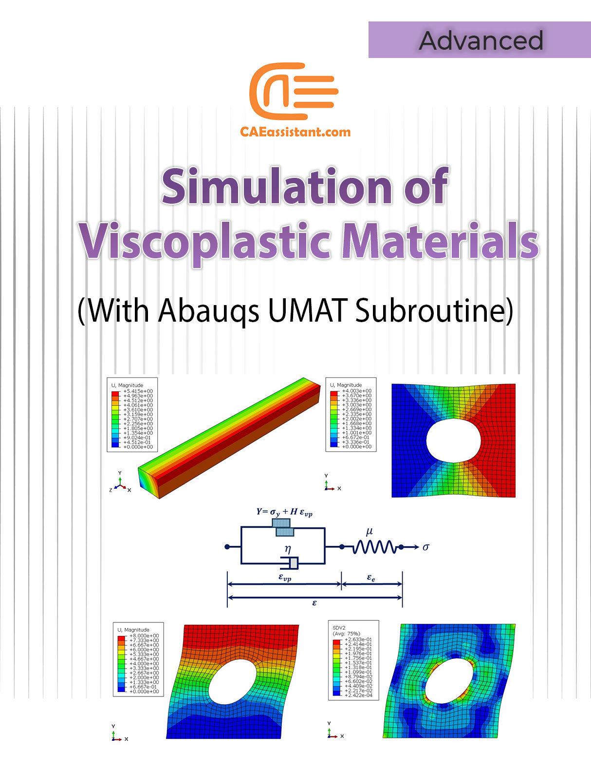
Perzyna Viscoplastic Model | UMAT Subroutine
Abaqus provides some built-in options for modelling rate-dependent plasticity (like Johnson–Cook or power-law hardening), but it does not directly include a general-purpose viscoplastic model. This can be a limitation when studying materials where time-dependent plastic flow is critical, such as metals at elevated temperatures, polymers, or soils.
To overcome this, Abaqus allows researchers to use the UMAT (User Material Subroutine) interface. With UMAT, you can directly implement the constitutive equations of any viscoplastic model to achieve viscoplastic material simulation.
There is a complete tutorial for this theory and its UMAT subroutine line by line in our full tutorial package:
What is the Perzyna Viscoplastic Model?
Many different models have been proposed by researchers to model viscoplastic materials, but one of the most efficient models is the Perzyna model.
The Perzyna viscoplastic model is a way to describe how materials deform when the plastic flow depends on time. In classical plasticity, once the stress reaches the yield surface, plastic deformation starts immediately, like flipping a switch. However, in reality, many materials such as metals, polymers, and soils do not yield instantly but instead deform gradually.
The Perzyna model accounts for this by introducing the concept of overstress, which means how far the stress is beyond the yield surface. If the stress is below the yield surface, the response is purely elastic. If the stress slightly exceeds the yield surface, plastic flow begins but at a slow rate. As the overstress increases, the rate of viscoplastic strain also increases.
In simple terms, the Perzyna model makes the yield surface act more like a soft boundary than a rigid wall, allowing plastic deformation to develop progressively over time depending on the level of stress.
Why Choose the Perzyna Model?
- Captures rate dependence: Unlike classical plasticity, it accounts for how strain rate affects yielding.
- Smooth transition: Avoids sharp yielding; useful in numerical simulations for stability.
- Applicable to many materials: Especially useful for metals under high strain rates, soils, and polymers.
- Numerical robustness: Helps reduce convergence issues in finite element simulations compared to purely rate-independent plasticity.
Formulas of the Perzyna Model
The Perzyna viscoplastic model is generally expressed as:
- Total strain rate decomposition:

where is the elastic strain rate, ![]() and
and ![]() is the viscoplastic strain rate.
is the viscoplastic strain rate.
- Viscoplastic strain rate (flow rule):

- Overstress function:

where:
 is the yield function,
 is reference stress,
 is the viscosity parameter (controls rate sensitivity),
- N is the rate-sensitivity exponent,
- ⟨⋅⟩ is Macaulay brackets (only positive values contribute).
This means that when the stress is inside the yield surface (f<0), no viscoplastic flow occurs; when outside, viscoplastic strains evolve depending on the overstress. The rheological model for the Perzyna model is as follows, because this model is viscoplastic, but the equations related to friction, damping, and elasticity can be different from other viscoplastic models.

Figure 6: Rheological model for the Perzyna model
Recap
In this article, we looked at viscoplasticity and how it can be modelled in Abaqus. Viscoplasticity describes materials that deform over time depending on both stress and loading duration, which makes it different from purely plastic or viscous behaviours.
This subject is important because many real materials, such as metals at high temperatures, polymers, soils, and asphalt, show time- and rate-dependent deformation. Understanding viscoplasticity helps engineers make better predictions about material performance under real loading conditions.
We first explained what viscoplasticity is, showing how it combines plasticity and viscosity. Then we covered Abaqus viscoplastic models, where we saw that Abaqus does not have a single viscoplastic option but uses tools like rate-dependent plasticity, creep, and viscous behaviour to capture these effects. After that, we introduced rheological modelling, which uses simple mechanical elements like springs, dashpots, and sliders to illustrate how different behaviours combine.
Finally, we explained the Perzyna viscoplastic model and how it can be implemented in Abaqus to account for gradual, time-dependent yielding.
Overall, we learned that Abaqus provides several ways to handle viscoplasticity, but for advanced cases, user subroutines like UMAT are needed. The Perzyna model is one of the most practical choices because it captures time-dependent plastic flow clearly and effectively.
The CAE Assistant is committed to addressing all your CAE needs, and your feedback greatly assists us in achieving this goal. If you have any questions or encounter complications, please feel free to share it with us through our social media accounts including WhatsApp.
Explore our comprehensive Abaqus tutorial page, featuring free PDF guides and detailed videos for all skill levels. Discover both free and premium packages, along with essential information to master Abaqus efficiently. Start your journey with our Abaqus tutorial now!