
What Are UMAT and VUMAT in Abaqus? Abaqus UMAT (User Material) and Abaqus VUMAT are Fortran-based subroutines used to define custom constitutive material models in Abaqus/Standard and Abaqus/Explicit, respectively. They allow engineers and researchers to program advanced mechanical behaviors—such as complex elasticity, plasticity, and composite damage—when built-in Abaqus material libraries are insufficient.
This CAE Assistant guide provides a definitive roadmap for developing, implementing, and executing these subroutines. By exploring input/output architectures, step-by-step coding for elastic and orthotropic models, and a direct UMAT vs. VUMAT comparison, readers will gain the practical expertise needed to write accurate custom algorithms. Access the provided free PDF guides and Fortran code templates to accelerate advanced material modeling projects.
UMAT / VUMAT Video Walkthrough
UMAT / VUMAT Audio Podcast
| Subroutine Type | Solver Interface | Primary Output Variables | Key Input Variables | Jacobian Requirement | Application Use Case | Vectorization Support | State Variables (SDV) Capacity |
|---|---|---|---|---|---|---|---|
| UMAT | Abaqus/Standard (Implicit) | STRESS, DDSDDE, STATEV, SSE, SPD, SCD | STRAN, DSTRAN, PROPS, TIME, DTIME, TEMP, DFGRD0, DFGRD1 | Required (consistent tangent stiffness) | Static, plasticity, creep, viscoelasticity | Not vectorized | *DEPVAR (NSTATV) |
| VUMAT | Abaqus/Explicit | STRESSNEW, STATENEW, ENERINTERNNEW, ENERINELASNEW | STRAININC, PROPS, DENSITY, DEFGRADOLD, STRESSOLD | Not required | Impact, crash, large deformation | NBLOCK vectorized | *DEPVAR (NSTATEV) |
What Are UMAT and VUMAT in Abaqus?
Abaqus comes with many built-in materials, but in real projects these are often not enough. That is why engineers use user subroutines. With Abaqus UMAT and Abaqus VUMAT, you can write your own material model in Fortran and link it directly to the solver. In simple terms, you are teaching Abaqus how your material reacts when it deforms.
Think of it like this: every time Abaqus takes a step, it calls your subroutine and asks, “What is the updated stress, and how should the material respond?” In a UMAT, this happens inside the implicit solver (Abaqus/Standard). In a VUMAT, it happens inside the explicit solver (Abaqus/Explicit).
-
UMAT: Runs with Abaqus/Standard, best for static or slow-loading problems. It also provides the material Jacobian (tangent stiffness), which makes convergence faster.
-
VUMAT: Runs with Abaqus/Explicit, ideal for dynamic events such as crash, impact, or large deformation. It updates stresses in blocks for many points at once.

Figure 1: UMAT subroutine workflow
Typical learning path
If you are starting from scratch, the usual path is simple:
-
Begin with a basic elastic model (so you can learn the structure and test your setup).
-
Add complexity step by step—plasticity, hardening, or viscoelastic behavior.
-
Once you’re comfortable, extend your code to include damage, failure, or rate-dependent effects.
-
Finally, try porting your UMAT logic into a VUMAT when your problem involves dynamics or large deformations.
This blog will guide you through that first step: writing and testing a minimal elastic UMAT, and then showing how the same idea extends to a VUMAT. By the end, you’ll know not just the theory but also the workflow needed to grow into more advanced models.

How to Prepare for Writing Abaqus Subroutines
Before you start coding an Abaqus UMAT or Abaqus VUMAT, there are a few basics you need to have in place. Don’t worry—you don’t need to be a Fortran wizard or a full-time theorist. But a solid foundation makes your life much easier.
1) Know Your Material Model Theory:
The most important step is to clearly understand the theory behind your material model. For example, if you are implementing elasticity, you should know the stress–strain law and how stiffness is defined. If you are implementing plasticity, you should know the yield function, flow rule, and hardening law. Without this, you won’t know if an error comes from the theory or the code.
2) Core Finite Element Concepts:
Since UMAT and VUMAT work at the integration point level, you need to be familiar with:
-
Stress and strain increments
-
State variables (history variables carried between increments)
-
Jacobian/tangent stiffness (DDSDDE Matrix) (important in UMAT for convergence)
3) Tools You’ll Need:
Finally, you need a proper coding environment:
-
A working Fortran compiler (Intel oneAPI is common today): Read this FREE blog to learn how to work with Fortran “Abaqus Fortran “Must-Knows” for Writing Subroutines“
-
Abaqus installed and linked to the compiler: read this blog to learn how to link Abaqus and Fortran “Abaqus Fortran Linking“
-
A text editor or IDE for coding (simple editors like Notepad++ or Visual Studio Code work fine)
With these basics ready, you can move smoothly into coding your first UMAT or VUMAT without unnecessary roadblocks.

DDSDDE Matrix & Newton-Raphson Method | Why They Matter?
In Abaqus/Standard, the solution is obtained using an iterative scheme known as the Newton-Raphson method. At each increment, Abaqus tries to satisfy equilibrium by updating displacements and stresses. The DDSDDE matrix plays a key role in this process. It represents the sensitivity of stress to strain changes. In simple terms, it tells the solver:
If strain changes slightly, how will stress respond?
A correct DDSDDE leads to:
- Faster convergence
- Fewer iterations
- More stable simulations
On the other hand, an inaccurate DDSDDE can cause:
- Slow convergence
- Divergence errors
- Excessive increment cutbacks
For nonlinear materials (plasticity, damage), DDSDDE must be consistent with the integration algorithm, not just an approximation.
Abaqus UMAT Variables: Interfaces, Inputs, and Outputs:
When you write an Abaqus UMAT, you are essentially filling in a contract: Abaqus passes certain variables into your code, you use them to compute the material response, and then you return results back to Abaqus. Understanding this data exchange is the first big step to feeling comfortable with user subroutines.
At every increment, Abaqus sends the current strain, time, material constants, and state variables to UMAT. Your job is to:
-
Use this information to compute the new stress and tangent stiffness.
-
Update history variables if the material has memory (plasticity, damage, etc.).
-
Send these results back to Abaqus so the analysis can continue.
Quick Cheat Sheet (Big Picture First)
Before diving deep, let’s take a look at a quick overview of the variables you’ll face when writing an Abaqus UMAT.
The official documentation classifies UMAT parameters into three groups:
-
Variables to be defined: what you must calculate and return (e.g., STRESS, DDSDDE).
-
Variables passed in for information: what Abaqus provides for you to use (e.g., STRAN, DSTRAN, PROPS).
-
Variables that can be updated: hybrid variables you can evolve over time (e.g., STATEV, energy variables).
But we made it simple for you:
| Category | Key Variables | What They Do |
|---|---|---|
| Inputs (given by Abaqus): passed in for information | STRAN, DSTRAN, PROPS, COORDS, TIME, DTIME, NDI, NSHR, NTENS, TEMP, PREDEF | Abaqus provides total strain, strain increment, material properties, coordinates, analysis time, and extra fields. |
| Outputs (you define): to be defined | STRESS, DDSDDE | You compute and return the stress tensor and tangent stiffness matrix. |
| Updatable | STATEV, SSE, SPD, SCD, RPL, DDSDDT, DRPLDE, DRPLDT | You evolve history variables and energy measures as the material response develops. |
Tip: Keep this table handy when you first start coding. It helps you quickly identify what Abaqus gives you and what you need to return.
Consistent Jacobian and Convergence
Your UMAT must return an accurate Jacobian matrix (DDSDDE) to ensure fast convergence,. This matrix represents the change in stress relative to the change in strain,. A “consistent” Jacobian allows the Abaqus/Standard solver to achieve quadratic convergence,. Consequently, the simulation finishes much faster. If you approximate this matrix, you might experience a loss of convergence speed or even solver failure.
UMAT Interface and Flow of Data
A UMAT always starts with the same subroutine declaration. It may look overwhelming at first, but it’s simply the “communication contract” between your code and Abaqus:
Explain that Abaqus sends info → UMAT processes it → returns updated stress & tangent → Abaqus continues. (See figure 1 again)
You can see and copy the Abaqus UMAT interface here or directly copy it from the Abaqus Documentation.
SUBROUTINE UMAT(STRESS,STATEV,DDSDDE,SSE,SPD,SCD,
     1 RPL,DDSDDT,DRPLDE,DRPLDT,
     2 STRAN,DSTRAN,TIME,DTIME,TEMP,DTEMP,PREDEF,DPRED,CMNAME,
     3 NDI,NSHR,NTENS,NSTATV,PROPS,NPROPS,COORDS,DROT,PNEWDT,
     4 CELENT,DFGRD0,DFGRD1,NOEL,NPT,LAYER,KSPT,JSTEP,KINC)
C
      INCLUDE 'ABA_PARAM.INC'
C
      CHARACTER*80 CMNAME
      DIMENSION STRESS(NTENS),STATEV(NSTATV),
     1 DDSDDE(NTENS,NTENS),DDSDDT(NTENS),DRPLDE(NTENS),
     2 STRAN(NTENS),DSTRAN(NTENS),TIME(2),PREDEF(1),DPRED(1),
     3 PROPS(NPROPS),COORDS(3),DROT(3,3),DFGRD0(3,3),DFGRD1(3,3),
     4 JSTEP(4)


      user coding to define DDSDDE, STRESS, STATEV, SSE, SPD, SCD
      and, if necessary, RPL, DDSDDT, DRPLDE, DRPLDT, PNEWDT


      RETURN
      END
Inputs (given by Abaqus): Variables Passed in for Information
These are the values Abaqus provides to your subroutine. You use them to compute the material response, but you do not overwrite them:
-
STRAN, DSTRAN: total strain and strain increment for the current step.
-
PROPS, NPROPS: material property values and their count.
-
TIME, DTIME: total analysis time and current increment length.
-
COORDS: spatial coordinates of the integration point.
-
NDI, NSHR, NTENS: number of direct, shear, and total stress/strain components (NTENS = NDI + NSHR). For example, that is 6 for a general 3D and 4 for a simplified plane strain (2D) model.
-
TEMP, DTEMP: current temperature and temperature increment.
-
PREDEF, DPRED: predefined field variables and their increments.
-
DFGRD0, DFGRD1, DROT: deformation gradient at start and end of increment, plus incremental rotation.
-
CELENT: characteristic element length (useful in softening/damage models).
-
NOEL, NPT, LAYER, KSPT, KSTEP, KINC: bookkeeping identifiers (element, point, step, increment).
Note. There are many other variables that Abaqus pass into UMAT and are not discussed here. According to your material, you may need to use them either.
Outputs: Variables to Be Defined or Updated
Inside UMAT, your job is to compute or update these variables:
-
STRESS (NTENS): This array is passed in as the stress tensor at the beginning of the increment and must be updated in this routine to be the stress tensor at the end of the increment. For a general 3D model, we need 6 values for stress (3 normal and 3 shear) so this vector will have 6 elements.
- DDSDDE(NTENS,NTENS): material Jacobian (tangent stiffness), needed for implicit solver convergence. A 2D format of Jacobian matrix with NTENS row and NTENS column.For small-deformation problems (e.g., linear elasticity) or large-deformation problems with small volume changes (e.g., metal plasticity), the consistent Jacobian can be calculated as:
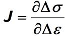 Where, ∆σ is the increment in (Cauchy) stress and ∆ε is the increment in strain. The variable DDSDDE(I,J) in the context of DDSDDE Abaqus UMAT specifies how the Ith stress component changes at the end of the time increment due to a tiny perturbation of the Jth component in the strain increment array.As you may guess, calculation of the consistent Jacobian or DDSDDE matrix can be the main challenge in writing a UMAT. This article provides a set of guidelines that will make the process of writing DDSDDE UMAT easier for you. An effective recommendation is to define variables for the elements of the DDSDDE matrix. This can make your code more organized.
 - STATEV: state variables (history-dependent quantities like plastic strain, damage, etc.).An array containing the Solution-Dependent state Variables (SDV). Abaqus pass in these parameters as the values at the beginning of the increment and at the end, return them as the values at the end of the increment. NSTATV (number of solution-dependent state variables associating with this material type) define the size of the array.We should specify the number of needed state variable (if any) when defining our model through Abaqus/CAE in Property module (we will discuss more, later).After completing the analysis, Abaqus can visualize the values of state variables (named as SDV1, SDV2, … in Abaqus/CAE) calculated during increments.
-
SSE, SPD, SCD: strain energy, plastic dissipation, and creep dissipation.
-
RPL: creep strain rate (if modeling creep).
-
DDSDDT, DRPLDE, DRPLDT: temperature-dependent derivatives (used if you include thermo-mechanical or creep effects).
-
PNEWDT: optional time increment control (if your material requires a smaller step).
Abaqus VUMAT Variables: Interfaces, Inputs, and Outputs
While UMAT works in the implicit solver, Abaqus VUMAT is the counterpart for the explicit solver. That means it is tailored for highly dynamic problems like crash simulations, high-speed impacts, or forming processes where wave propagation and inertia dominate.
Instead of updating one integration point at a time like UMAT, a VUMAT processes many integration points in a batch. This improves efficiency in explicit dynamics, but also means you need to structure your code slightly differently.
The philosophy stays the same: Abaqus provides strains, state variables, and material constants; your code returns stresses, updated state, and energies. But since explicit dynamics doesn’t require the tangent stiffness, there’s no DDSDDE.
Figure 2 shows how Abaqus and VUMAT work together by sharing and updating important material variables. Here’s a simple breakdown of the process: Abaqus hands over the old variables—like stress, temperature, and any state-dependent variables—that describe the current state of the material. These serve as the starting point for VUMAT’s calculations.
Using custom equations, VUMAT takes these inputs and calculates new values for stress, temperature, and other state variables. Once VUMAT has processed this information, it sends the updated variables back to Abaqus for further analysis and to keep the simulation going smoothly.
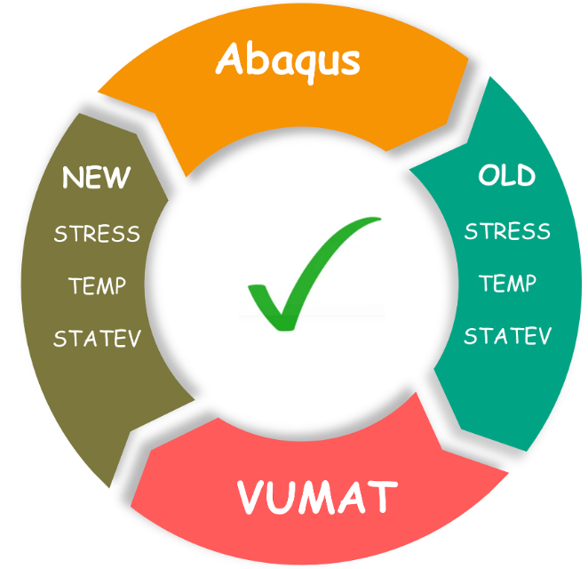
Figure 2: How VUMAT work
Quick Cheat Sheet for VUMAT (Big Picture First)
Abaqus/Explicit calls VUMAT with the old state (stressOld, stateOld, energies, etc.), the kinematic updates (strainInc, relSpinInc, defgradOld/New, stretchOld/New), and step info.
Your job: compute stressNew, stateNew, and optionally enerInternNew and enerInelasNew, for each material point in the block. Then Abaqus continues the time march.
Here’s the snapshot of what VUMAT deals with:
| Category | Key Variables | What They Do |
|---|---|---|
| Inputs (given by Abaqus): passed in for information | strainInc, relSpinInc, defgradOld, stretchOld, stressOld, stateOld, props, density, coordMp, charLength, tempOld, fieldOld, enerInternOld, enerInelasOld, stepTime, totalTime, dtArray, jInfoArray | All the data Abaqus provides: strain increments, spin, deformation measures, material constants, old stresses, old state vars, old energies, temperature/fields, geometry, and time info. |
| Outputs (you define): to be defined | stressNew, stateNew | You must return the updated Cauchy stress and the new state variables. |
| Updatable | enerInternNew, enerInelasNew | If your model tracks energy, update internal energy and inelastic energy per unit mass. |
Tip: Keep this table handy when you first start coding. It helps you quickly identify what Abaqus gives you and what you need to return.
VUMAT Interface and Flow of Data
Abaqus/Explicit gives you the old stress, state, energies, deformation measures, strain increments, spin, and fields.
You must compute and return the new stress, new state variables, and optionally the new energies.
You can see and copy the Abaqus VUMAT interface here or directly copy it from the Abaqus Documentation.
subroutine vumat(
C Read only (unmodifiable)variables -
     1  nblock, ndir, nshr, nstatev, nfieldv, nprops, jInfoArray,
     2  stepTime, totalTime, dtArray, cmname, coordMp, charLength,
     3  props, density, strainInc, relSpinInc,
     4  tempOld, stretchOld, defgradOld, fieldOld,
     5  stressOld, stateOld, enerInternOld, enerInelasOld,
     6  tempNew, stretchNew, defgradNew, fieldNew,
C Write only (modifiable) variables -
     7  stressNew, stateNew, enerInternNew, enerInelasNew )
C
      include 'vaba_param.inc'
      parameter (i_info_AnnealFlag = 1,
     *     i_info_Intpt    = 2, ! Integration station number
     *     i_info_layer  = 3, ! Layer number
     *     i_info_kspt   = 4, ! Section point number in current layer
     *     i_info_effModDefn = 5, ! =1 if Bulk/ShearMod need to be defined
     *     i_info_ElemNumStartLoc   = 6) ! Start loc of user element number
C
      dimension props(nprops), density(nblock), coordMp(nblock,*),
     1  charLength(nblock), dtArray(2*(nblock)+1), strainInc(nblock,ndir+nshr),
     2  relSpinInc(nblock,nshr), tempOld(nblock),
     3  stretchOld(nblock,ndir+nshr),
     4  defgradOld(nblock,ndir+nshr+nshr),
     5  fieldOld(nblock,nfieldv), stressOld(nblock,ndir+nshr),
     6  stateOld(nblock,nstatev), enerInternOld(nblock),
     7  enerInelasOld(nblock), tempNew(nblock),
     8  stretchNew(nblock,ndir+nshr),
     8  defgradNew(nblock,ndir+nshr+nshr),
     9  fieldNew(nblock,nfieldv),
     1  stressNew(nblock,ndir+nshr), stateNew(nblock,nstatev),
     2  enerInternNew(nblock), enerInelasNew(nblock), jInfoArray(*)
C
      character*80 cmname
C
      pointer (ptrjElemNum, jElemNum)
      dimension jElemNum(nblock)
C
      lAnneal = jInfoArray(i_info_AnnealFlag)
      iLayer = jInfoArray(i_info_layer)
      kspt   = jInfoArray(i_info_kspt)
      intPt  = jInfoArray(i_info_Intpt)
      iUpdateEffMod = jInfoArray(i_info_effModDefn)
      iElemNumStartLoc = jInfoArray(i_info_ElemNumStartLoc)
      ptrjElemNum = loc(jInfoArray(iElemNumStartLoc))

      do 100 km = 1,nblock
        user coding
  100 continue

      return
      end
Inputs (given by Abaqus): Variables Passed in for Information
Abaqus groups arguments you must not overwrite. Here’s how that maps to what you use inside the material update:
-
Problem size and indexing
-
nblock: number of material points you must update in this call. The nblock variable, unlike UMAT, which is called separately for each material point, VUMAT receives information for a group of material points as input, and the code should update all of them. The number of these points is stored in the nblock variable. -
ndir,nshr: number of direct and shear components; total tensor size isndir + nshr. -
nstatev,nfieldv,nprops: lengths for state variables, user fields, and material constants. -
jInfoArray: flags and indices (e.g., integration point, layer, section point, anneal flag).
-
-
Time controls
-
stepTime,totalTime,dtArray: step time, total time, and stable time-increment data. Use these if your model is rate-dependent.
-
-
Geometry & material data
-
coordMp,charLength: point coordinates and characteristic length (often used in damage). -
props(nprops): your Abaqus UMAT/VUMAT material constants from the Property module. For example, in the VUMAT subroutine, the material properties (props) and other variables like density should be correctly indexed and used. If you have variables like E (Young’s modulus), (Poisson’s ratio), and yield (yield stress), make sure they correspond to the correct props array indices. -
density(nblock): current density passed in for each point.
-
-
Kinematics and fields
-
strainInc(nblock, ndir+nshr): strain increment for this step. The Strainlnc variable as input contains the strain increment(the strain increment typically refers to the change in strain between two consecutive steps or increments in a simulation.) for the change in the strength tensor during these increments. The name of the material defined in the GUI is passed to VUMAT by Cmname. -
relSpinInc(nblock, nshr): incremental spin (useful for objective stress update). -
defgradOld/New,stretchOld/New: deformation gradient and stretch measures (old and new). -
tempOld/New,fieldOld/New: temperature and user-defined field variables (old and new).
-
-
History at the start of increment
-
stressOld(nblock, ndir+nshr):Stress tensor at each material point at the beginning of the increment(fig 13). The stress state of the material at the start of the increment is used as the initial reference for the calculations in the VUMAT subroutine. The material’s response is then updated based on this initial stress state as the simulation progresses, and the stress is modified throughout the increment depending on the material behavior you define within VUMAT. -
stateOld(nblock, nstatev): State variables at each material point at the beginning of the increment. -
enerInternOld(nblock),enerInelasOld(nblock): starting energies per mass.
-
Notes for beginners
• The shear components’ order follows Abaqus conventions tied tondir/nshr. Map indices carefully.
•propsindexing is yours to define in CAE; document it at the top of your code.
• You will usually loopdo km = 1, nblockand read/write the km-th row of each array.
Outputs (you define): Variables to Be Defined or Updated
These are the values you produce for each material point:
-
Variables to be defined (write-only)
-
stressNew(nblock, ndir+nshr): Cauchy stress at end of increment. The most important variable that should be defined at the end of the increment. This variable holds the stress at the integration point. The subroutine uses this value to calculate how the material resists deformation. -
stateNew(nblock, nstatev): updated solution-dependent state variables. State variables are an array where we can save values to use in the next increment. The length of this array is defined in the GUI. These are state variables that describe the material’s internal state, like plastic strain, damage, or any history-dependent variables. For example, in a plasticity model, you might have a state variable that tracks the accumulated plastic strain.
(These two are mandatory in almost all models.)
-
-
Variables that can be updated (write-only)
-
enerInternNew(nblock): internal energy per mass stored elastically (etc.). -
enerInelasNew(nblock): dissipated inelastic energy per mass (e.g., plastic work, damage).
(Set them if your model needs energy tracking or you plan to review energy balances.)
-
Common mistakes to avoid
• Don’t write into*_Oldarrays,tempNew,defgradNew,fieldNew, etc.; they are inputs here.
• Don’t return engineering shear strains as stress—stressNewis Cauchy stress in vector form.
• Never assumenblock = 1. Always loop.
✅ The Most Crucial Output: The DDSDDE Matrix
Among all UMAT outputs, DDSDDE is the most critical one for implicit analysis.
While stress (STRESS) defines the current material state, DDSDDE controls how efficiently Abaqus can reach that state. Think of it this way:
STRESS → tells Abaqus “where you are”
DDSDDE → tells Abaqus “how to get there faster”
A poorly defined DDSDDE may still produce correct results, but:
- Simulation time increases significantly
- Convergence becomes unreliable
For advanced models (plasticity, viscoelasticity), deriving DDSDDE analytically is strongly recommended.
Numerical Stability and Integration Methods
Writing a UMAT requires more than just defining a stress-strain law. You must transform constitutive rate equations into incremental forms. Most experts prefer the Backward Euler (implicit) integration method for UMAT,. This method is unconditionally stable. However, it often requires local iterations like the Newton-Raphson method,. In contrast, the Forward Euler (explicit) method is simpler but has a stability limit. If your strain increment exceeds this limit, the results will fail.
How to Write Your First UMAT Subroutine in Fortran
When learning Abaqus UMAT for the first time, it helps to practice with well-structured benchmark problems. here, we present two examples which you can start writing your first UMAT subroutine with and the step-by-step tutorial of both examples are available to you in FREE UMAT tutorial PDF file.
here we just see the problem descripotion and the subroutines of the examples:
Geometry: a 50×50×400 solid beam modeled with C3D8 elements. Boundary conditions: one end fixed, the other end given a displacement in the longitudinal direction. Material: isotropic linear elasticity (E, ν). Purpose: verify that a UMAT elastic implementation matches Abaqus’s built-in Elastic material. Subroutine: standard isotropic elastic UMAT, where the stress update and stiffness matrix are coded explicitly.

SUBROUTINE UMAT(STRESS,STATEV,DDSDDE,SSE,SPD,SCD,
     1 RPL,DDSDDT,DRPLDE,DRPLDT,
     2 STRAN,DSTRAN,TIME,DTIME,TEMP,DTEMP,PREDEF,DPRED,CMNAME,
     3 NDI,NSHR,NTENS,NSTATV,PROPS,NPROPS,COORDS,DROT,PNEWDT,
     4 CELENT,DFGRD0,DFGRD1,NOEL,NPT,LAYER,KSPT,JSTEP,KINC)
C
      INCLUDE 'ABA_PARAM.INC'
C
      CHARACTER*80 CMNAME
      DIMENSION STRESS(NTENS),STATEV(NSTATV),
     1 DDSDDE(NTENS,NTENS),DDSDDT(NTENS),DRPLDE(NTENS),
     2 STRAN(NTENS),DSTRAN(NTENS),TIME(2),PREDEF(1),DPRED(1),
     3 PROPS(NPROPS),COORDS(3),DROT(3,3),DFGRD0(3,3),DFGRD1(3,3),
     4 JSTEP(4)

      REAL*8 EMOD,ENU,EBULK3,EG2,EG,EG3,ELAM,ONE,TWO,THREE
	ONE=1.0
	TWO=2.0
	THREE=3.0
C ----------------------------------------------------------------
C UMAT FOR ISOTROPIC ELASTICITY
C CANNOT BE USED FOR PLANE STRESS
C ----------------------------------------------------------------
C PROPS(1) - E
C PROPS(2) - NU
C ----------------------------------------------------------------
C
       IF (NDI.NE.3) THEN
       WRITE (7, *) 'THIS UMAT MAY ONLY BE USED FOR ELEMENTS
     1 WITH THREE DIRECT STRESS COMPONENTS'
       CALL XIT
       ENDIF
C
C ELASTIC PROPERTIES
	 EMOD=PROPS(1)
	 ENU=PROPS(2)
	 EBULK3=EMOD/(ONE-TWO*ENU)
	 EG2=EMOD/(ONE+ENU)
	 EG=EG2/TWO
	 EG3=THREE*EG
	 ELAM=(EBULK3-EG2)/THREE
	 print*,'ELAM',ELAM
C
C ELASTIC STIFFNESS
C
	 DO K1=1,NDI
	 DO K2=1,NDI
	 DDSDDE(K2,K1)=ELAM
	 END DO
	 DDSDDE(K1,K1)=EG2+ELAM
	 END DO
	 DO K1=NDI+1, NTENS
	 DDSDDE(K1,K1)=EG
	 END DO
C
C CALCULATE STRESS
C
	 DO K1=1, NTENS
	 DO K2=1, NTENS
	 STRESS(K2)=STRESS(K2)+DDSDDE(K2,K1)*DSTRAN(K1)
	 END DO
	 END DO
C
      RETURN
      END
Want to learn how to implement these cases? Get free access to these tutorials and 11 specialized workshops in our Free UMAT & VUMAT course.

Geometry: a 2D plane stress element representing a composite lamina. Material: orthotropic elasticity with three independent constants. Extra feature: failure is evaluated using the Tsai–Hill criterion inside UMAT. Purpose: show how UMAT can handle more advanced material behavior than Abaqus’s built-in library. Subroutine: orthotropic stress–strain law with additional failure check coded in Fortran.

SUBROUTINE UMAT(STRESS,STATEV,DDSDDE,SSE,SPD,SCD,
     1 RPL,DDSDDT,DRPLDE,DRPLDT,
     2 STRAN,DSTRAN,TIME,DTIME,TEMP,DTEMP,PREDEF,DPRED,CMNAME,
     3 NDI,NSHR,NTENS,NSTATV,PROPS,NPROPS,COORDS,DROT,PNEWDT,
     4 CELENT,DFGRD0,DFGRD1,NOEL,NPT,LAYER,KSPT,JSTEP,KINC)
C
      INCLUDE 'ABA_PARAM.INC'
C
      CHARACTER*80 CMNAME
      DIMENSION STRESS(NTENS),STATEV(NSTATV),
     1 DDSDDE(NTENS,NTENS),DDSDDT(NTENS),DRPLDE(NTENS),
     2 STRAN(NTENS),DSTRAN(NTENS),TIME(2),PREDEF(1),DPRED(1),
     3 PROPS(NPROPS),COORDS(3),DROT(3,3),DFGRD0(3,3),DFGRD1(3,3),
     4 JSTEP(4)
      REAL*8 E1,E2,V12,V21,G12,D11,D22,D66,CFULL(3,3),Y,X,Z,R,F11,F22,
     1F12,F66,F1,F2,F6,XT,XC,YT,YC,SU12

C=================================================================================
C                                 GIVE PROPS
C=================================================================================

      E1=PROPS(1)
      E2=PROPS(2)
      V12=PROPS(3)
      G12=PROPS(4)
      XT=PROPS(5)
      XC=PROPS(6)
      YT=PROPS(7)
      YC=PROPS(8)
      SU12=PROPS(9)
      PRINT*,' E2', E2
      V21=(E2/E1)*V12
      R=1.0/(1.0-(V12*V21))
      D11=E1*R
      D22=E2*R
      D66=G12
      D12=E2*V12*R
C=================================================================================
C                     FILL DEGRADED STIFNESS MATRIX
C=================================================================================

      DO K1=1,3
        DO K2=1,3
            DDSDDE(K2,K1)=0.0
        END DO
      END DO
      DDSDDE(1,1)=D11
      DDSDDE(1,2)=D12
      DDSDDE(2,2)=D22
      DDSDDE(1,3)=0.0
      DDSDDE(2,3)=0.0
      DDSDDE(3,3)=D66
      DDSDDE(2,1)=D12
      DDSDDE(3,1)=0.0
      DDSDDE(3,2)=0.0

C=================================================================================
C                             CALCULATE STRESS
C=================================================================================
         DO I=1,3
          Z=0.0
           DO J=1,3
           Z=Z+DDSDDE(I,J)*DSTRAN(J)
           END DO
          STRESS(I)=STRESS(I)+Z
         END DO

C=================================================================================
C                          TSAI-HILL CRITERIA
C=================================================================================

        IF (STRESS(1).GE. 0.0)THEN
            X=XT
        ELSE
            X=XC
        END IF
        IF (STRESS(2).GE. 0.0)THEN
            Y=YT
        ELSE
            Y=YC
        END IF

        F11=1.0/(X**2.0)
        F1=0.0
        F12=-1.0/(2.0*(X**2.0))
        F22=1.0/(Y**2.0)
        F2=0.0
        F66=1.0/(SU12**2.0)
        F6=0.0
C       FAILURE SURFACE
        F=F11*(STRESS(1))**2+F22*((STRESS(2))**2)+F66*((STRESS(3))**2
     1)+2.0*F12*STRESS(1)*STRESS(2)+F1*STRESS(1)+F2*STRESS(2)+F6*
     2STRESS(3)
        STATEV(1)=SQRT(F)

      RETURN
      END
Using Abaqus Utility Routines
Do not code everything from scratch. Abaqus provides built-in utility routines to simplify complex tasks,. For example, use ROTSIG to rotate tensor state variables during large-strain analysis,. Furthermore, you can use SINV to calculate stress invariants or SPRIND for principal directions,. These tools reduce coding errors and maintain technical depth.
Implementation in Abaqus & Compilation
After successfully developing the UMAT, the code must be incorporated into Abaqus to correctly compile a working Abaqus analysis. When defining the Abaqus job, you can add the developed UMAT. After Submitting the job, the UMAT will be compiled into a working executable by Abaqus automatically and can then be used to run the FEA simulation.
After normally defining your FEM model in Abaqus/CAE, generally, you need to pass 4 more steps within Abaqus/CAE to incorporate a UMAT in your analysis:
1. Define a User Material
Say Abaqus that you will use a UMAT as a material model. You can also use other material models of Abaqus if there is no intervention. For example, you can use Abaqus’s own model for elasticity but develop a UMAT to model a very specific plasticity model.
From Property module, when defining a material, from General tab select User Material. That is all you should do.
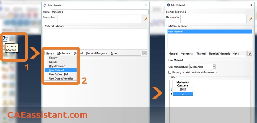
Figure 3: Define User-Material in Abaqus CAE
2. Define inputs (Mechanical Constants) for UMAT in Abaqus
When you select User Material as a material model for your problem, you can add as many constants as you wish in Data section. Type under Mechanical Constants the values you want to pass into written UMAT. After entering any data, you can press Enter to add a new row. These values then will be accessible through UMAT via PROPS array (PROPS(1), PROPS(2),…).
3. Define the No. of state variables
Many mechanical constitutive models may require the storage of Solution-Dependent state Variables (SDV) such as plastic strains, back stress, saturation values, etc. in rate constitutive forms or historical data for theories written in integral form. You should allocate storage for these variables in the associated material definition. There is no restriction on the number of state variables.
The number of such variables required at the points is entered as part of the material definition. In Abaqus/CAE, Property module when defining a material, from General tab select Depvar. Then select the required quantity in Number of solution-dependent state variables.
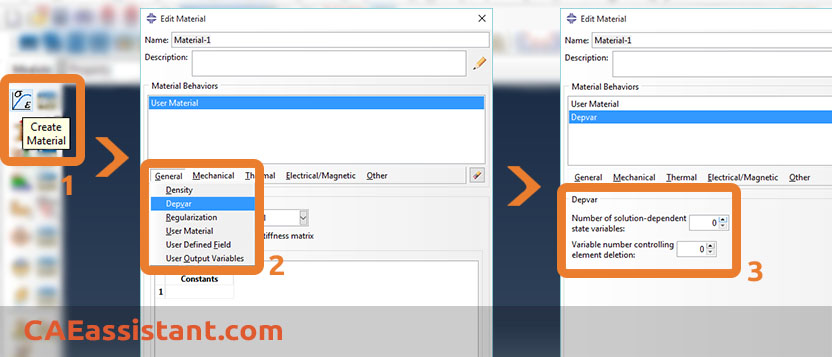 Figure 4: Defining Depvar in Abaqus/CAE UMAT in Abaqus
State variables can be output to the output database (.odb) file using output identifiers SDV. You can ask Abaqus to visualize them later after completion of the job. In Step module, after defining your analysis type, from Field Output Manager, you can edit the F-Output-1 created automatically by Abaqus:
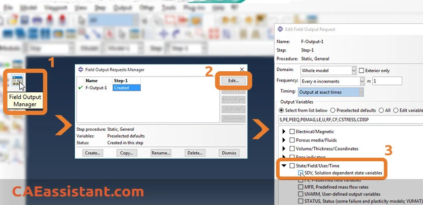
Figure 5: Requesting SDV in Field Output
Remember that the SDV in Abaqus/CAE is exactly the same as STATEV in Abaqus Subroutine Interface. That is just a difference in naming by developers of Abaqus.
4. Give the Path of UMAT to Abaqus
Like any other subroutine, when creating an Abaqus job, you should provide the path of the UMAT to Abaqus. Abaqus can then read the subroutine and update the DDSDDE matrix per iteration. You can include one or more UMATs in a model by specifying the name of a Fortran source file that contains the subroutines.
EXAMPLE: Isotropic Linear Elastic Material (Implementation)
As we will discuss in section 6 (Examining UMAT results), at first, we start from a very simple model like simple tension (displacement-based) on one-element mode. After building our FEM model in Abaqus/CAE like any other model without UMAT, we should (we do not need any state variable in this simple UMAT):
1. Define a User Material from the Property module
2. Define two Mechanical Constants as inputs for our elastic model UMAT: E and Nu
3. Give the Path of our written UMAT to Abaqus when defining the job.
5. Testing and debugging UMAT Abaqus subroutine
Keep in mind that writing a UMAT in Abaqus is exactly like developing a piece of code in Fortran. So, when you finish typing your code, the main task starts! After the first run, you may encounter compiling errors, complaining by compiler about structures DDSDDE Matrix or nested loops of DDSDDE Matrix and so on. Be patient; this is really normal even for experienced UMAT developers.
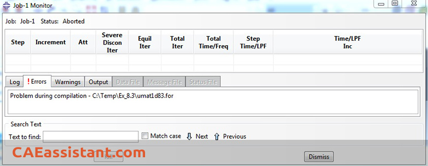
Figure 6: Problem during compilation Error in Job Monitor
When you are facing an error and you are not sure about the cause, in a most easygoing manner, you can check the values by using write command to write the variable values into .msg file. We will discuss most important Fortran commands that are really handy when writing a UMAT Abaqus (and also any subroutine) in an article later.
Common UMAT Errors and How to Fix Them
When working with UMAT in Abaqus, many errors are not general solver issues, but are directly related to how the material model is implemented. Below are some real and frequently observed UMAT-specific problems:
| Error / Issue | Typical Symptom | Root Cause | Practical Solution |
|---|---|---|---|
| Non-Convergence (Too many attempts) | Analysis stops or requires many increments | Inconsistent DDSDDE matrix with stress update | Derive DDSDDE analytically and ensure consistency with return mapping |
| Stress Not Updating Correctly | Constant or unrealistic stress response | Misuse of STRAN instead of DSTRAN | Use DSTRAN for incremental updates and validate with uniaxial test |
| STATEV Not Updating | No plasticity or damage evolution | State variables not stored correctly | Update STATEV at the end of UMAT and check indexing |
| Instability in Plastic Models | Oscillating stress or divergence | Incorrect integration algorithm | Use implicit schemes (e.g., Backward Euler) and enforce consistency condition |
| Incorrect Stiffness Response | Model too stiff or too soft | Wrong DDSDDE or incorrect material parameters | Verify PROPS values and compare with analytical solution |
| Works in Simple Test but Fails in Real Model | Passes single element test but fails in complex model | Missing multiaxial behavior or coupling effects | Test under multiaxial loading and validate full tensor behavior |
Advanced Subroutine Modeling
Ready to go past linear elasticity? Great. Here’s a clear path to extend your Abaqus UMAT and Abaqus VUMAT to real-world behavior—without getting lost.
Add realistic physics step by step:
Plasticity (small strain → finite strain)
-
Start with a simple J2/von Mises model. Build a trial stress, check yield, perform return mapping, and update plastic strain + hardening.
-
For UMAT, always provide a consistent tangent (
DDSDDE). For VUMAT, focus on stable updates overDTIME. -
Later, extend to finite strain plasticity using the deformation gradient and objective stress updates.
Damage and failure
-
Introduce a damage variable and degrade stiffness: $$\sigma = (1 – D)\sigma_{eff}$$
-
Use the
charLengthvariable in Abaqus VUMAT to regularize softening. -
Add deletion criteria for elements once failure is reached.
Viscoelasticity / rate dependence
-
Implement Maxwell or Prony series with internal variables.
-
In UMAT, add algorithmic tangents; in VUMAT, integrate rate forms carefully.
Hyperelasticity
-
Derive stress from a strain-energy function and handle finite strain.
-
Often easier in VUMAT where the deformation gradient is given directly.
Handling large strains and strong nonlinearities
-
Use the correct kinematic frame (
DFGRD0/DFGRD1in UMAT,DEFGRADin VUMAT). -
Rotate stresses with spin increments to avoid drift.
-
In UMAT, Newton convergence depends on a consistent tangent; use
PNEWDTto suggest cutbacks. -
In VUMAT, stability depends on
DTIME; reduce increment size for accuracy.
Rule of thumb: Use UMAT for quasi-static problems that need fast convergence. Use VUMAT for impact, crash, and progressive failure where stability matters more than convergence speed.
Reliable development workflow
-
Run unit tests on a single element.
-
Perform load–unload path checks.
-
Do mesh refinement studies for softening models.
-
Track energy balance (elastic, plastic, damage).
-
Always compare against theory or a built-in Abaqus material.
Where to read next
If you want to dive deeper, here are the most useful resources:
-
NASA White Paper: Core Crush Modeling → advanced VUMAT for progressive composite damage in explicit simulations.
-
Oxford Innovation VUMAT project page → academic resources and open VUMAT development.
-
Technia Abaqus page → overview of Abaqus Unified FEA and how user subroutines fit in.
-
Textbooks:
-
Computational Inelasticity (Simo & Hughes) — algorithms for plasticity and tangents.
-
Nonlinear Finite Elements for Continua and Structures (Belytschko et al.) — large-strain methods.
-
For industry-grade VUMAT, read the NASA white paper.
For academic research, Oxford Innovation’s page is a solid reference.
Abaqus UMAT vs VUMAT: Which User Subroutine Should You Choose?
If you’ve followed along so far, you know both Abaqus UMAT and Abaqus VUMAT let you define custom materials. But which one should you use? The answer depends on the physics of your problem and the solver you plan to run.
-
UMAT (User MATerial) → works with Abaqus/Standard (implicit solver).
-
VUMAT (Vectorized UMAT) → works with Abaqus/Explicit (explicit solver).
In other words:
-
UMAT is all about Newton iterations and requires a consistent tangent matrix for convergence.
-
VUMAT skips the tangent and updates stress explicitly at every increment.
Side-by-side comparison
| Feature | UMAT (Implicit) | VUMAT (Explicit) |
|---|---|---|
| Solver | Abaqus/Standard (quasi-static, implicit dynamics) | Abaqus/Explicit (dynamic, impact, crash) |
| Stability | Relies on Newton convergence; tangent matrix critical | Conditionally stable; step size depends on wave speed & element size |
| Tangent stiffness | Must provide DDSDDE (consistent tangent) | Not required |
| Typical applications | Metal plasticity, creep, viscoelasticity, small strain, quasi-static loading | Impact, crash, contact, progressive damage, composites |
| Handling failure | Works, but can struggle with localization | Commonly used; element deletion supported |
| Control knobs | PNEWDT for time step cutbacks, tangent accuracy | Reduce DTIME, smooth material updates |
| Debugging effort | Higher (due to tangents & convergence) | Lower (no tangent, but careful with stability) |
When to choose UMAT
Use UMAT when:
-
Your problem is quasi-static or low-speed dynamics.
-
You need fast convergence with an implicit solver.
-
Material requires a consistent tangent operator (e.g., elastoplasticity with hardening).
-
Large step sizes are desired, and stability is less of a concern.
Examples:
-
Metal plasticity under slow forming.
-
Creep and viscoelasticity in steady processes.
-
Thermo-mechanical coupled simulations in Standard.
When to choose VUMAT
Use VUMAT when:
-
Your problem is highly nonlinear with contact, damage, or impact.
-
You want to simulate fracture, progressive failure, or crashworthiness.
-
You prefer not to deal with tangents and Newton convergence.
-
Time step stability is manageable (explicit usually requires many increments).
Examples:
-
Composite crash (see the NASA white paper on composite crushing).
-
Impact of automotive or aerospace structures.
-
Large deformation problems where implicit would fail to converge.
How to decide
A quick decision chart:
-
If you want accuracy in quasi-static problems → go UMAT.
-
If you want robustness in highly nonlinear dynamic problems → go VUMAT.
That’s why many beginners start with UMAT to learn the structure, then move to VUMAT for real-world crash or failure modeling.
VUMAT Vectorization with NBLOCK
To maximize VUMAT performance, you must write vectorized code. Abaqus/Explicit processes material points in large blocks, usually defined by the variable NBLOCK,. Therefore, you should avoid branching or IF statements inside your loops,. Branching prevents the compiler from vectorizing the routine. This slows down the analysis significantly. Additionally, always use the state-old and state-new architecture correctly to ensure data integrity across increments.
Conclusion
We’ve come a long way. You now know:
-
What Abaqus UMAT and Abaqus VUMAT are, and why they matter.
-
How they differ, and when to choose one over the other.
-
The building blocks of inputs, outputs, and data flow.
-
How to write and run your first elastic UMAT step by step.
-
Where to go next with plasticity, damage, viscoelasticity, or composites.
If you follow this path, you’ll move from a beginner writing a simple elastic law to an advanced user implementing plasticity, damage, or even progressive failure in composites.
Your roadmap forward:
-
Start with elastic UMAT (as we did here).
-
Add internal variables and test simple plasticity.
-
Move to larger strain and nonlinear models.
-
Explore VUMAT for explicit crash and impact problems.
Final note
Learning UMAT and VUMAT is not just about coding — it’s about building confidence in custom material modeling. The more you test, compare, and validate, the faster you’ll grow.
Abaqus UMAT & VUMAT FAQs
UMAT stands for User Material. We use User Material when none of the existing material models included in the ABAQUS material library accurately represents the behavior of the material to be modeled. We use a UMAT in the stress calculation step to obtain the stress tensor. In the process, Abaqus also need to define the (consistent) Jacobian to continue its incremental scheme.
Generally, to write a newly developed UMAT, you should first master all the aspects of the constitutive model for your material. Then, get Familiar with UMAT Abaqus parameters (Inputs/Outputs). In the next step, develop and implement the FORTRAN code of the UMAT in Abaqus. At last, the UMAT subroutine should be tested and debugged to find accurate UMAT results.
All parameters for a UMAT are divided into 4 distinguished groups:
Parameters that are available by Abaqus like STRESS, STRAN, DSTRAN, TIME, and DTIME.
Parameters that are calculated and updated by UMAT, like STRESS and DDSDDE Matrix.
Parameters are entered through the Abaqus model definition and sent to UMAT. These parameters are indicated by PROPS.
Solution-Dependent State Variables Parameters that require to be stored. These parameters are indicated by PROPS STATEV.
After normally defining your FEM model in Abaqus/CAE, you need to define a User Material in the Property module. Then, Type under Mechanical Constants the values you want to pass into written UMAT to define inputs. These values will then be accessible through UMAT via the PROPS array (PROPS(1), PROPS(2),…). After that, if the mechanical constitutive model needs the storage of solution-dependent state variables, select the required quantity in the number of SDV. At last, Give the Path of UMAT to Abaqus.
Always start verifying the UMAT with a small model to study quality in the developed material model. You can run a couple of examples to verify the compiled UMAT in Abaqus and compare the results against analytical, experiment or semi-analytical (predicted) results.
Did you know that you can use UMAT in Comsol Multiphysics? interesting, isn’t it? well, you can learn all about it for FREE in our blog:





 English
  Korean
  Chinese
7 Responses
Excellent article! We will be linking to this particularly great article on our website. Keep up the great writing. Kanya Waite Longo
Really informative blog article. Really thank you! Cool. Kattie Lorenzo Harwin
You made some nice points there. I looked on the internet for the subject matter and found most individuals will agree with your site.
Hello! I could have sworn I’ve been to this blog before but after browsing through some of the post I realized it’s new to me. Anyways, I’m definitely happy I found it and I’ll be book-marking and checking back frequently!
i like this fabulous article
Simply want to say your article is as astounding. The clearness to your post is
simply spectacular and i could think you’re an expert on this subject.
Fine with your permission allow me to grasp your
feed to stay up to date with approaching post. Thank you 1,000,000 and please carry on the
rewarding work.