
To model Concrete Damage Plasticity (CDP) effectively, you need a precise mix of elastic, plastic, and damage parameters—most of which can be found in validated research data like the SCDP tables or specialized UHPC calibrations; but we made it easy for you and we have it all in this blog.
Whether you are analyzing a standard reinforced concrete beam, pushing the limits of Ultra-High Performance Concrete (UHPC), or trying to preserve historical masonry, getting the parameters right is the difference between a realistic crack pattern and a complete numerical meltdown.
In this guide, we skip the theoretical fluff and give you the exact step-by-step workflow to calibrate your materials, implement element deletion, and finally fix those frustrating convergence errors. Let’s turn your crashing models into accurate, publishable results.
Why is Concrete Behavior So Hard to Predict?
Concrete is a “quasi-brittle” composite material that acts very differently under tension versus compression. So you need models like the concrete damage plasticity model because standard linear models cannot capture the complex cracking and crushing that define structural failure.
- Compression: Concrete demonstrates high strength under compression, but once a certain stress threshold is exceeded, it begins to show nonlinear behavior, marked by cracking and crushing.
- Tension: Concrete is relatively weak under tensile stress, where its nonlinear response is largely governed by the initiation and spread of cracks.
- Shear: Nonlinear behavior in shear arises from the interaction between cracks and the interlocking of aggregates.
Additionally, factors such as loading rate, temperature, moisture levels, and the presence of reinforcement significantly influence the nonlinear behavior of concrete.
Concrete is not a simple solid. Instead, it is a heterogeneous mix of aggregates, cement paste, and water. Because of this, its nonlinear behavior starts at the meso-scale. This means that internal voids and the interaction between stones and paste determine how the material breaks.
When you use Concrete damage plasticity, you are combining two powerful theories. First, the plasticity part handles the permanent deformation when concrete is crushed under high pressure. Second, the damage part tracks how the material loses its stiffness as cracks spread.
Abaqus Concrete Damage Plasticity Model
The failure criterion in the plastic range of the material is expressed under combined stresses. This criterion is divided into two main categories based on the material’s response to hydrostatic pressure.
In most materials, ductile behavior is known as hydrostatic pressure-dependent, and non-metallic materials such as soil, rocks, and concrete belong to this category and are pressure-dependent.
Speacking of soil; you can learn how to model soils in our blog “Abaqus Soil Modeling | Key Models and Applications“.
When discussing the Abaqus Concrete Damage Plasticity Model, the failure potential function is derived from the Drucker-Prager model for concrete behavior.
The main formulation of the plastic potential surface in the CDP model is represented by Equation 1, and the three-dimensional shape of the deviation from the stress planes is shown on the meridian planes, as presented in Figure 1.

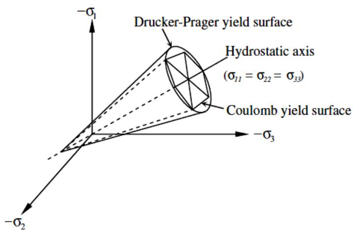
Figure 1: Drucker-Prager model [3]
The principles of failure, introduced by Kachnov in the mid-1950s, were based on the reduction of stress surfaces. Since then, the failure mechanism has been considered based on degradation models and is currently evaluated using the secant of damage softening.
Degraded models consider the elastic stiffness degradation as the total damage. For concrete, this behavior is defined based on the degree of confinement of the element. When the confinement is low due to the loading process, damage occurs rapidly and is irreversible. Conversely, if the confinement is high, more time is needed for damage to develop when the load is applied.
The formula for the elastic damage softening model in scalar dimension d is given by Equation 2.

Implementation of CDP model in Abaqus CAE
To use the Concrete Damage Plasticity model in Abaqus, simply go to the Property module and create a new material. In the edit material window, select Mechanical. Then click on Plasticity. Now, you can select the Concrete Damage Plasticity model. This process is shown in Figure 2.
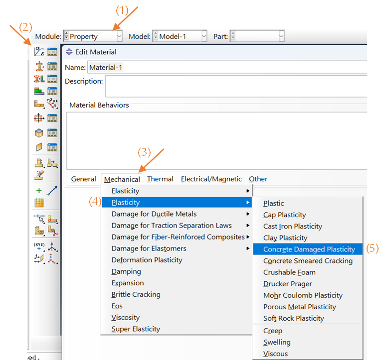
Figure 2: Implementation of the CDP model in Abaqus
After selecting CDP, in the Plasticity section, you can define the parameters of the Concrete Damage Plasticity model in Abaqus based on the characteristics of the desired concrete. These parameters are explained in the next section, and the corresponding values are provided.
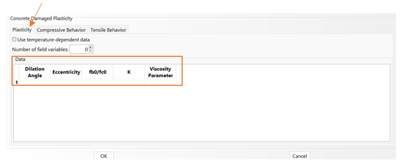
Figure 3: Defining the plasticity data for CDP model in Abaqus
For the Compressive Behavior, as shown in Figure 4, you need to define the compressive stresses and inelastic strains for your model. Additionally, by selecting the Suboptions, you can define the damage based on inelastic strains. In the following sections of the article, we provide a detailed explanation of how to calculate these components and their significance.
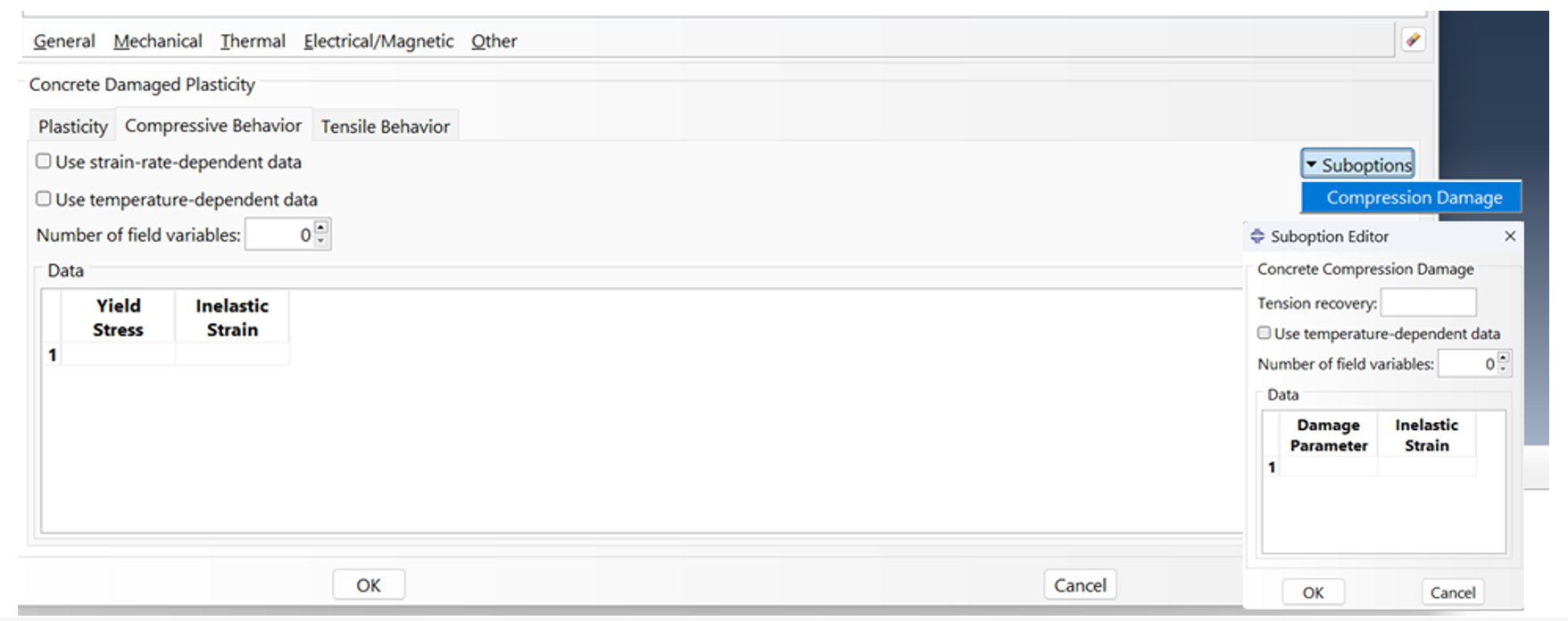
Figure 4: Defining the compressive behavior for CDP model in Abaqus
As illustrated in Figure 5, for the tensile behavior, it’s necessary to specify the tensile stresses and cracking strain values for your model. Additionally, you can use the Suboption to define damage based on cracking strains. The upcoming sections of the article offer a comprehensive explanation of how to calculate these parameters and their importance.
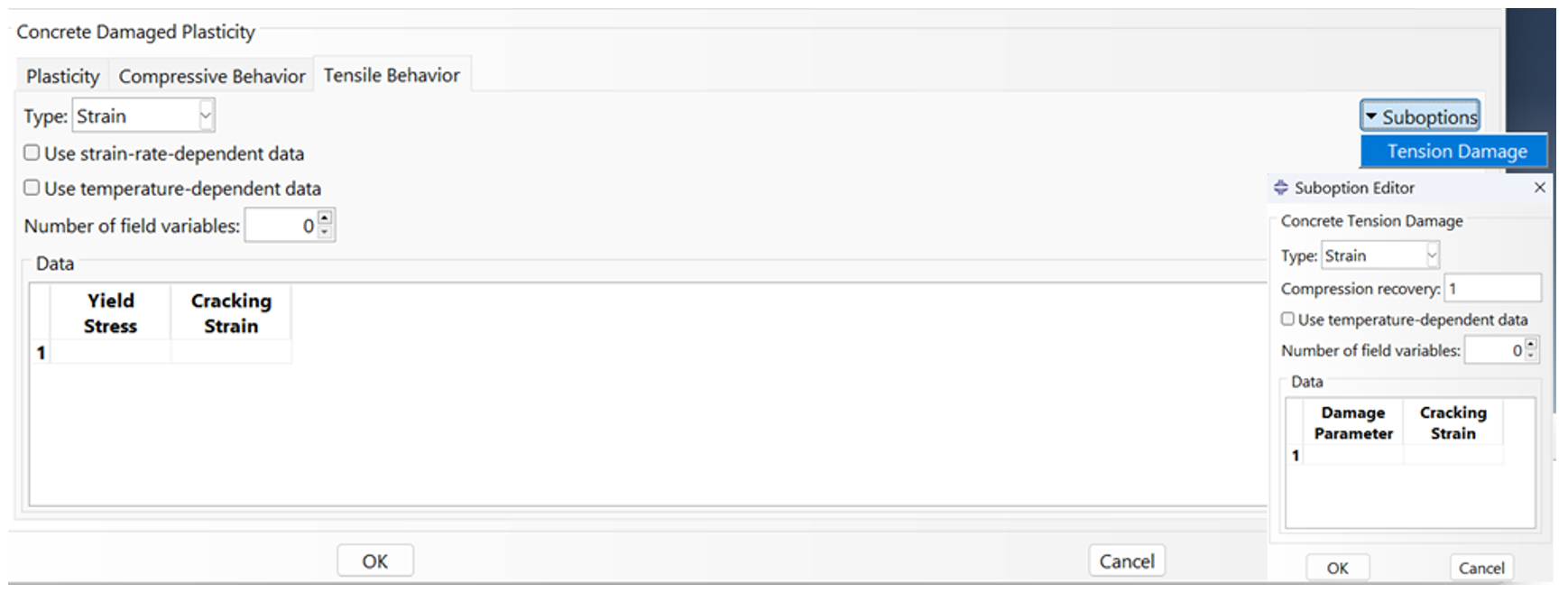
Figure 5: Defining the tensile behavior for CDP model in Abaqus
What are the Required Parameters for CDP Model in Abaqus
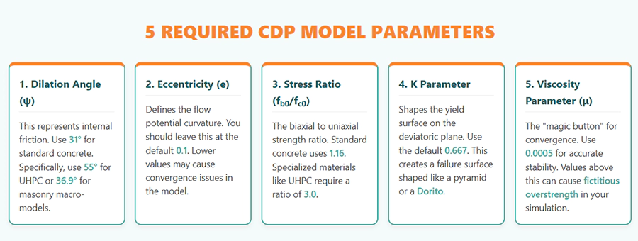
To define Concrete damage plasticity correctly, you must enter five specific parameters in the “Plasticity” tab (see figure 3 above):
- Dilation Angle (ψ)
- Viscosity Parameter (
 )
) - K Parameter
- Eccentricity (e)
- Stress Ratio (
 )
)

The dilation angle and viscosity parameter are the most critical settings in the Abaqus concrete damage plasticity model. Consequently, these two values determine if your simulation will converge or produce unrealistic material strength.
- Dilation angle
This represents the internal friction angle of the material. For standard reinforced concrete, researchers recommend values between 30° and 40°. A smaller dilation angle results in more brittle material behavior, while a larger angle leads to behavior resembling that of ductile materials.
Specifically, a value of 31° is often considered optimal. However, if you are modeling Ultra-High Performance Concrete (UHPC), you should increase this to 55°.
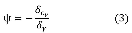
Essentially, the dilation angle represents the correlation between volumetric strain and shear strain, as indicated by equation (3). Based on Vermeer and de Borst’s research, materials that are sensitive to hydrostatic pressure, such as rock, soil, and concrete, have a typical dilation angle of about 20°, which exceeds their internal friction angle, typically around 12°, under multiaxial stress conditions.
- Viscosity parameter
Think of this as the “magic button” for convergence. Abaqus sets this to zero by default, but this often causes the analysis to crash. To improve stability, you should use an optimum value of 0.0005. Furthermore, you must keep this value as small as possible. If the viscosity is too high, it creates “fictitious overstrength” that makes your concrete look stronger than it actually is.
- K Parameter
This ratio defines the shape of the yield surface on the deviatoric plane. You should use the default value of 0.667(or 2/3). This shapes the failure surface like a three-dimensional pyramid, which looks like a Dorito chip in a 2D view.
- Eccentricity
This small positive number defines the rate at which the flow potential approaches its asymptote. You should almost always leave this at the default value of 0.1.
Values of m that are significantly less than the default value may lead to Abaqus convergence issues if the material is subjected to low confining.
- Stress Ratio ()
This is the ratio of biaxial compressive yield stress to uniaxial yield stress. For standard concrete, the default is 1.16. However, for specialized materials like UHPC, research suggests a much higher ratio of 3.
[/vc_column_text][/vc_column][/vc_row]
How to Prepare Your Test Data for Abaqus CDP Model?
You must convert “Total Strain” from your lab tests into inelastic strain (for compression) or cracking strain (for tension). If you paste raw laboratory data directly into the Abaqus concrete damage plasticity model, the simulation will immediately abort.
To define Concrete damage plasticity, you first need your material’s Modulus of Elasticity ( ). Specifically, you must use these two formulas in your spreadsheet to prepare your data:
Isolate Permanent Deformation:
To define Concrete damage plasticity, you must use your material’s Modulus of Elasticity (E0) to remove the elastic portion from your total strain. Specifically, these formulas isolate the permanent deformation for Abaqus.
Compression: Inelastic Strain
ε̃cin = εc – (σc / E0)
Tension: Cracking Strain
- E0: Initial Modulus of Elasticity
- σ: Uniaxial Stress (Test Data)
- ε: Total Strain (Test Data)
- σ / E0: Elastic portion to be removed
Why Raw Test Data Causes an Abaqus Abort?
Raw test data includes the initial elastic branch. However, the Abaqus concrete damage plasticity model only starts recording data from the onset of plastic deformation. If you include the elastic part in the Plasticity tab, Abaqus will think your plastic strain is zero while stress is still changing.
Internally, the software must compute a specific plastic strain value from your inputs. Using raw data creates a mathematical conflict, which causes the solver to crash during the first few increments.
The “Golden Rule”: Positive and Monotonically Increasing
Before running your analysis, check your columns in Excel. You must satisfy two strict criteria:
- Values must be positive: Plastic strain cannot be a negative number.
- Values must be monotonically increasing: Every value in your strain column must be larger than the one before it.
If your strain values drop or stay the same as stress decreases, Abaqus will throw a “negative plastic strain” error. Furthermore, ensuring this “monotony” is the best way to prevent the “Too many attempts” error in highly nonlinear simulations.
Expert CDP Data Rules:
- The Yield Point Rule: Specifically, your data in the Plasticity tab must start exactly at the onset of plastic deformation. Consequently, the first row of your strain column (Inelastic or Cracking) must always be 0.
- Troubleshooting Tip: If the E0 used in your spreadsheet formulas does not perfectly match the Modulus of Elasticity in your Abaqus settings, your calculated strains might become negative. If this happens, Abaqus will throw an error and abort the simulation immediately.
The “Spring & Clay” Analogy:
Think of concrete like a spring attached to a piece of clay. When you pull it, the spring stretches (elastic) and the clay deforms (plastic). The abaqus concrete damage plasticity model only wants to know how much the clay itself stretched permanently. If you include the spring’s movement in your data, the software gets confused and stalls the engine.
Modeling Stiffness Degradation (Damage & Recovery)
While the stress-strain tables define the material’s strength, they do not tell Abaqus how the material’s stiffness should degrade as it fails. To simulate the physical “weakening” of the concrete, you must implement the Damage sub-option. This is critical for any simulation involving unloading, reloading, or cyclic behavior where the material does not return to its original elastic state.
Estimating Damage Without Lab Data: Ideally, damage parameters are obtained from complex cyclic loading tests. However, if you only have standard uniaxial test data, you can use approximation formulas to estimate the scalar damage variables. These variables represent the percentage loss of elastic stiffness, ranging from 0 (undamaged) to 1 (total loss of strength).
The Logic of Stiffness Recovery: Concrete has a unique “healing” property: when a tensile crack closes under compression, the material regains its ability to carry a load. In the abaqus concrete damage plasticity model, this is controlled by the recovery parameters ( and
and  ). Setting these correctly ensures your model accurately captures this “crack-closure” effect during load reversals.

- The “0 to 1” Rule: Damage variables must range from 0 (undamaged) to 1 (failed). Values in your Excel must be positive and monotonically increasing. If damage decreases as strain increases, Abaqus will abort the simulation.
Physical Analogy: Micro-Cracks & Exhaustion
If the “Strain Math” was about measuring how much the clay permanently stretched, these Damage Parameters are about measuring how many micro-cracks have formed in the material’s internal structure.
Damage tells Abaqus that the material is “exhausted” and can no longer hold the same load it once did, even if the strain remains the same.
You can watch this video for more detail about this matter:
What If I DO NOT Have Test Data for CDP Model? | Validated SCDP Tables
For researchers who do not have specific laboratory test data, the Simplified Concrete Damage Plasticity (SCDP) model provides validated, tabulated values for standard concrete grades.
If you lack experimental stress-strain curves, you can use these SCDP parameters. In these standards, “B” stands for Beton (concrete), and the number represents the maximum compressive strength in MPa. These tables provide the exact Yield Stress and Inelastic/Cracking Strain values required for the Abaqus Plasticity and Damage sub-options.
Validated SCDP Material Tables
| Concrete Grade | E₀ (GPa) | Peak (MPa) | Yield (MPa) | Inelastic Strain |
|---|---|---|---|---|
| B20 | 21.2 | 20 | 10.2 | 0 |
| 15.0 | 0.000173 | |||
| 20.0 | 0.000937 | |||
| 10.2 | 0.002800 | |||
| B30 | 26.6 | 30 | 15.3 | 0 |
| 22.5 | 0.000119 | |||
| 30.0 | 0.000828 | |||
| 15.3 | 0.002800 | |||
| B40 | 30.0 | 40 | 20.4 | 0 |
| 30.0 | 0.000080 | |||
| 40.0 | 0.000746 | |||
| 20.4 | 0.002800 | |||
| B50 | 33.4 | 50 | 25.5 | 0 |
| 37.5 | 0.000041 | |||
| 50.0 | 0.000667 | |||
| 25.5 | 0.002800 |
- Standard Plasticity Parameters for All Grades:
– Dilation Angle: 31°
– Eccentricity: 0.1
– fb0/fc0: 1.16
– K: 0.67
– Viscosity: 0
- Data Sources & Additional Reference:
The values in these tables were derived from the Simplified Concrete Damage Plasticity (SCDP) model. For a complete dataset and more in-depth analytical models, please refer to the following original research publication:
Simplified Damage Plasticity Model for Concrete (Hafezolghorani et al.)
Some Notes
- Strain Origin: Note that for every grade, the inelastic strain starts at 0 when the yield stress is first reached.
- Tensile Strength: In the SCDP model, the initial tensile strength (
 ) is typically assumed to be 10% of the peak compressive strength (e.g., 3.0 MPa for grade B30).
 - Reliability: This simplified approach (SCDP) has been verified against 3D nonlinear finite element models and empirical formulations, showing excellent correlation for beams and columns.

Specialized Calibration for UHPC (Ultra-High Performance Concrete)
When modeling Ultra-High Performance Concrete (UHPC), the standard parameters used for conventional concrete will often lead to premature failure or inaccurate stress distribution. This is because UHPC lacks coarse aggregates (reducing shear interlock) and contains steel fibers that create a significant tensile bridging effect.
To capture the high ductility and triaxial strength of UHPC in the Abaqus concrete damage plasticity model, research by Fakeh et al. (2023) suggests a specialized calibration of the plasticity flow rules. Unlike standard concrete which typically uses a dilation angle of 30°–40°, UHPC requires a much higher dilation to account for its unique volume changes during plastic shearing.
 Note: It is important to remember that in the Abaqus concrete damage plasticity model, the biaxial stress ratio is denoted as
  in the software interface, while technical literature—including the studies on UHPC—often uses the notation
  .
.
CDP for Masonry Structures
While the Concrete Damage Plasticity (CDP) model was designed for concrete, it has become a standard for simulating the post-elastic behavior of masonry. To model a large-scale building, treating every brick and mortar joint individually (Micro-modeling) is computationally expensive. Instead, engineers use a Homogeneous Continuum approach, where the masonry is modeled as a single uniform material with equivalent properties.
The “Texture” Influence on Dilation ( )
)
A critical discovery in masonry research is the relationship between wall texture and the Dilation Angle ().
- In Micro-models: The dilation is typically low (around 20°) as it reflects the properties of the mortar alone.
- In Macro-models (Continuum): To match experimental results, the dilation angle must be significantly higher (often reaching 36.9°).
This is because the physical interlocking of bricks (the texture) creates a “granular” effect that induces higher dilatancy than the material would exhibit on its own. Without increasing dilation angle, a continuum model will show a premature loss of strength compared to real-world tests.
How to Simulate CDP Model Failure?
Since the Abaqus/CAE GUI does not currently have a dedicated field for material failure within the CDP window, this requires a manual Keyword Edit to the input file.
In standard Concrete Damage Plasticity (CDP) simulations, elements that reach 100% damage (d=1) stay in the model, often resulting in “stretching” or distorted meshes that look unrealistic. To simulate actual crushing or spalling where material is physically removed, you must activate Element Deletion.
The *CONCRETE FAILURE Keyword Edit
This command tells Abaqus at what specific strain levels an element should be considered “failed” and removed from the calculation.
- In the Model Tree, right-click on your model name and select Edit Keywords.
- Locate the material definition block (under *MATERIAL, NAME=CONCRETE).
- Directly below the *CONCRETE TENSION DAMAGE or *CONCRETE COMPRESSION DAMAGE data lines, insert the following block:

 : The tensile cracking strain at which the element fails.
 : The compressive inelastic strain at failure.
 and : The tensile and compressive damage variables (usually 0.99) at which the element is deleted.

 :
:  :
:  and
and  :
: Expert Instruction: Per the sources, you must input the values from the very last row of your material property tables. For example, using the B20 grade from our SCDP tables, the failure inelastic strain is 0.0035.
To obtain complete datasets for additional concrete grades (B30, B40, and B50), please refer to the primary research paper: Hafezolghorani et al. (2017) – “Simplified Damage Plasticity Model for Concrete” .
Enabling Deletion in the Mesh Module
Even with the keyword added, elements won’t disappear unless the mesh is told to allow it.
- Go to the Mesh Module and select Mesh > Element Type.
- Select your concrete part.
- In the dialog box, find Element Deletion and change the toggle to Yes.
Setting up the “Status” Field Output
To see the elements disappear in the Visualization module (ODB), you must request the Status variable.
- Go to Step Module > Output > Field Output Requests.
- Under the Failure/Fracture category, check the box for Status.
- Ensure DAMAGEC and DAMAGET are also selected for comprehensive crack tracking.
Ho to do a CDP Simulation in Abaqus? | Practical Walkthrough (The 2D Beam Example)
Even with perfect material parameters, a simulation can fail due to poor interaction definitions or numerical singularities at boundary conditions. For a 2D planar beam, two specific setup techniques are essential for accuracy and convergence.
- Reinforcing via the “Embedded Region” Constraint
In Abaqus, rebar is typically modeled using truss elements (wire parts) because they primarily resist axial tension and compression. However, simply placing the rebar inside the concrete instance is not enough; you must “lock” them together so they deform as a single unit.
- The Logic: Without a constraint, the concrete would deform while the rebar remains stationary in space.
- The Setup: Use the Embedded Region constraint found in the Interaction Module.
◦ Embedded Region: Select your steel rebar set.
◦ Host Region: Select the concrete beam part.
- Pro Tip: Create Sets for your rebar and concrete in the Assembly module before moving them together. This makes selecting them in the constraint menu much easier once the rebar is hidden inside the beam.
- Handling Stress Concentrations at Supports
Applying boundary conditions or loads directly to a single node in a 2D model creates mathematical singularities (infinite stress at a point), which often causes the solver to abort due to local concrete crushing.
- The Solution: Use Analytically Rigid Surfaces to represent supports or loading rollers.
- Implementation:
- Create the support as an Analytic Rigid part (usually a semi-circle or cylinder).
- Define a Reference Point (RP) for each support to control its movement or fixity.
- Establish Surface-to-Surface Interaction between the rigid support (Master) and the bottom of the beam (Slave).
- Set the Interaction Property to “Hard Contact” for normal behavior and “Frictionless” for tangential behavior.
Practical Interaction & Loading Tips
Embedded Region Constraint:
- Define Rebar as T2D2 (Truss) or B21 (Beam) elements.
- Set Rebar as Embedded Region and Concrete as Host Region.
- Ensure mesh seeds for rebar and concrete are compatible to avoid local distortions.
Analytical Rigid Surfaces:
- Avoid Nodal Constraints; use Rigid Supports to distribute reactions.
- Fix the RP (Reference Point) for translation and rotation.
- Apply Hard Contact to prevent the beam from penetrating the support.
Watch this Video for a step by step tutorial:
Common Issues and Troubleshooting
Now let’s see the most common issues in the way of CDP modeling in Abaqus and how to solve them:
- Solving the “Too Many Attempts” Error
This error occurs when the material’s non-linearity is so high—often due to sudden cracking—that the solver cannot find a stable mathematical state within the specified increment.
- The Numerical Lubricant: To bypass this, Abaqus provides a sub-option called Viscoplastic Regularization, governed by the Viscosity Parameter (
 ).
). - The Logic: Viscosity allows the stress state to momentarily exist “outside” the yield surface, smoothing the numerical response and allowing the solver to bypass local instabilities during failure.
- Optimal Setting: For standard reinforced concrete, a value of 0.0005 is considered optimal for balancing speed and accuracy. For more stable models or simple geometries, researchers often use 0.0001.
Pro Tip: For a deep dive into the mechanics of this error and more advanced solver settings, refer to this detailed guide on Too Many Attempts Made for This Increment.
- Why Stress Exceeds the Input Yield Stress?
Users often notice that their output stress ( ) is slightly higher than the yield stress (
 or
or  ) they entered in the property module.
- The Reason: This is a direct side effect of the Viscosity Parameter (). Because viscoplasticity allows the stress state to exist outside the yield surface to achieve convergence, the “over-stress” is the numerical price paid for a stable simulation.
- Validation: If the stress is significantly higher (more than 10-15%), it indicates your viscosity is too high.
- Avoiding “Fictitious Overstrength”
While increasing makes your model “sturdy” and easier to run, a value that is too high results in Fictitious Overstrength.
- The Risk: If is excessive, the model will show a peak load significantly higher than experimental data, and the softening branch will appear artificially smooth and ductile.
- Correction: Always run a sensitivity check. If your load-displacement curve changes significantly when you reduce , your current value is likely too high and is compromising the physical accuracy of the simulation.
Conclusion
Throughout this guide, we have moved from the basic elastic response to the complex math of softening regimes and viscoplastic regularization. We have seen how the dilation angle acts as a surrogate for aggregate interlocking in concrete and geometric texture in masonry macro-models.
Remember, a successful simulation isn’t just one that reaches the end of the time step—it’s one that maintains physical integrity. By using the SCDP tables for calibration, implementing the *CONCRETE FAILURE keyword for visuals, and tuning viscosity to bypass numerical instabilities, you are now equipped with a professional-grade workflow. Now, it’s time to submit your job and see the results for yourself.
Here we have presented some users questions about CDP or concrete damage plasticity:
I. CDP analysis
Q: I used the CDP model to create a small solid cubical part. After establishing the necessary boundary conditions, the load is applied. When I check at the stress in my odb file, some of the elements have more stress than the yield stress I entered? Is there an explanation for this?
A: Two things could have happened; either you didn’t enter the CDP parameters correctly, such as units might be wrong or anything else, or when you defined the compressive and tensile behavior, you didn’t control the slope of the diagrams.
Check the link below. In these lessons, you will understand the CDP completely.
Abaqus Tutorial for Beginners (Abaqus Tutorial for Civil Engineering)
II. Concrete Damage Plasticity Abaqus simulation
Q: In the Concrete Damage Plasticity Abaqus simulation, I’m working with fiber concrete. I had previously modeled the EN 14651 (3-point bending) test and now I was testing my “real” beams. She has longitudinal reinforcement and stirrups, as seen in the photo (figure 1). There are no stirrups in a small test area (I’m dealing with shear). However, regardless of how the material input stresses change, the force-displacement graphs in the post-peak zone show increasing force (Figures 2 and 3).
The supports were positioned in a beam region (without drawing the supports) and the displacement was applied in an RP with “coupling.” Reinforcement can also be found in the “embedded region.” I put it to the test with some random material from a YouTube video, and the strength keeps increasing. Is there something wrong with my model? In addition, the peak force is significantly higher than the experimental data. Figures 4 and 5 show the data from the CDP.
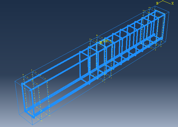
Figure 1
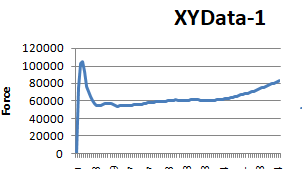
Figure 2
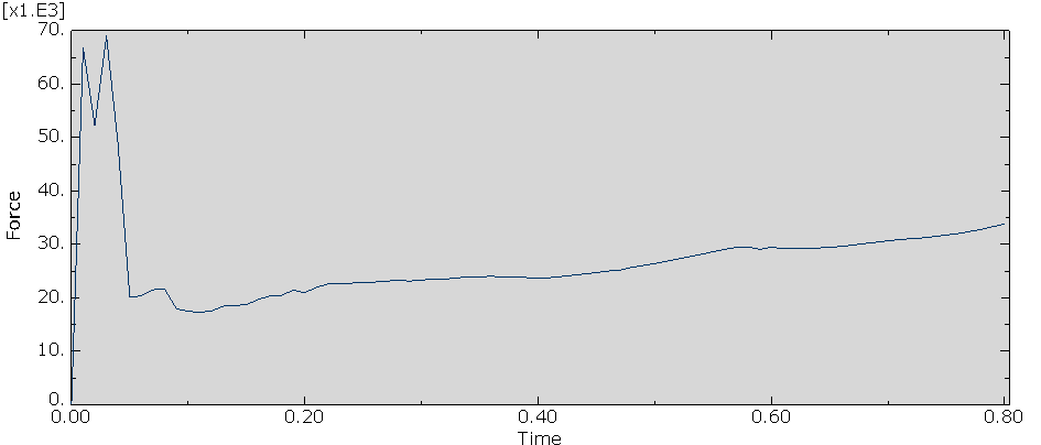
Figure 3
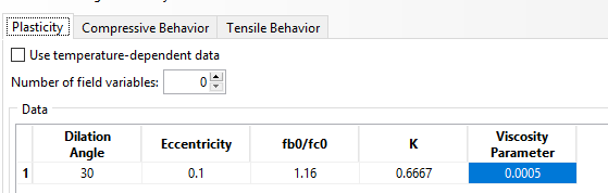
Figure 4
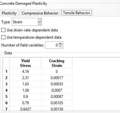
Figure 5
A: First of all, you cannot enter random material from a YouTube video and expect to get similar results to the experimental ones. The data you enter must match the ones in the experimental test.
Second, you need to check the data you use is True or engineering and must match the experimental data. If the stress data is True, the diagram you obtained might be correct.
The last thing I recommend is checking the input data units and rechecking your model; you might have done something wrong. I suggest referring to the link below as well. It might help you a lot.
Abaqus Tutorial for Beginners (Abaqus Tutorial for Civil Engineering)
III. Concrete damaged plasticity (CDP) model in Abaqus
Q: I created a CDP model with enlarged boundary elements for a shear wall. I performed a nonlinear static analysis with a 500 mm displacement. I couldn’t observe any difference in results when I increased the amount of longitudinal reinforcement in enlarged boundary elements (column). I mean that the longitudinal bar confinement effect is not visible.
How do I get the confinement effect of ties while modeling an RCC column in Abaqus?
A: I don’t know how you increased the column reinforcement. I suggest rechecking your model. Please note that increasing the number of the bars and decreasing their cross-section simultaneously could cause them to counteract each other’s effect; therefore, the stress won’t change. If that’s what you did, you should change one of them or if you want to change both, do it properly to see its effects in your model.
The CAE Assistant is committed to addressing all your CAE needs, and your feedback greatly assists us in achieving this goal. If you have any questions or encounter complications, please feel free to share it with us through our social media accounts including WhatsApp.
If you need deep training, our Abaqus Course offerings have you covered. Visit our Abaqus course today to find the perfect course for your needs and take your Abaqus knowledge to the next level!
Of course you can always learn more in detail about Abaqus in Abaqus Documentation.



 English
  Korean
  Chinese