Impact happens when two objects hit each other with a sudden force in a short amount of time. Impact dynamics covers how structures respond to sudden loads. Low velocity impact (≈1–10 m/s) typically causes indentation and delamination; high velocity impact (>100 m/s) produces inertial, wave and penetration effects.
By understanding both low and high velocity regimes within the broader field of impact dynamics, one can predict failure mechanisms, choose the right testing methods, and design more resilient materials.
In this blog, we start by introducing what impact means in mechanics and how it can be categorized in different ways, such as based on speed, duration, and the objects involved. We then explain key concepts like momentum, impulse, and the law of momentum conservation, along with how these relate to impact behavior and formulas. After building this foundation, we move on to how impacts are simulated using Abaqus.
| Type of Impact | Typical speed | Dominant mechanics | Common tests |
|---|---|---|---|
| Low-velocity impact | ≈ 1–10 m/s | Quasi-static deformation, delamination/indentation | Drop-weight, pendulum |
| High-velocity / ballistic | > 100 m/s | Wave propagation, shock, penetration | Gas gun, ballistic ranges |
| Hypervelocity impact | > 2000 m/s (>> speed of sound) | Extreme shock, plasma effects, severe fragmentation | Light-gas guns, space debris tests |
(Note: ranges depend on material, impactor mass and geometry — state these caveats where you cite sources.)
Impact Mechanics FAQ
Typically ~1–10 m/s; depends on mass and material—state the caveat.
Practical ballistic tests often exceed 100 m/s; aerospace/defense uses much higher ranges.
Impacts above ~2000 m/s, often relevant to space debris, cause extreme shock, plasma formation, and fragmentation.
Energy spreads into subsurface delamination without large surface cracks; surface may look minor but internal damage reduces residual strength.
Peak force, absorbed energy, indentation depth, residual velocity (for ballistic), and CAI residual strength.
What is Impact Dynamics in Mechanics?
Impact dynamics refers to the study of collisions or high-force events that occur over a short duration when two bodies collide with each other.
Impact dynamics is the study of how structures respond when energy is delivered over a short time — covering contact mechanics, energy transfer, strain‑rate dependent material behavior, and resulting damage or failure modes.

Figure 1: Metal spheres impacting in a Newton’s cradle [Ref]
The principles of momentum conservation, the coefficient of restitution, and impulse-momentum relationships constitute the foundation of impact dynamics.
These concepts enable engineers to forecast post-collision velocities, energy dissipation, and impact forces.
By gaining proficiency in these principles, students are equipped to address intricate real-world collision situations and devise creative solutions.
Basic Concepts of Impact Mechanics
In the realm of impact mechanics, it is essential to grasp several key concepts:
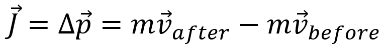
Impulse: This (J) is the product of force and the time over which it acts: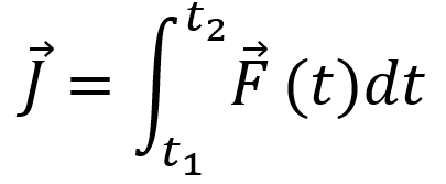
- Units: Newton-second (Ns)
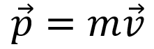
Momentum (Linear Momentum): This quantifies the motion of an object and is calculated as the product of its mass and velocity:
Coefficient of Restitution (e): A measure of how “bouncy” a collision is. The coefficient of restitution, e, is the ratio of the particles’ relative separation velocity after impact, to the particles’ relative approach velocity before impact. The coefficient of restitution is also an indicator of the energy lost during the impact.
The equation defining the coefficient of restitution, e, is:
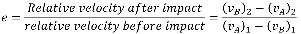
In general, e has a value between zero and one.
In a perfectly elastic collision (e = 1), no energy is lost and the relative separation velocity equals the relative approach velocity of the particles. In a plastic impact, (e = 0), the relative separation velocity is zero.
A thorough understanding of these principles is crucial for analyzing the behavior of various materials during an impact.
- : perfectly elastic
- 0<e<1: partially inelastic
- e=0: perfectly inelastic
Kinetic Energy: The energy an object possesses due to its motion, given by:
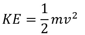 m is mass and v denote velocity.
Strain Rate Sensitivity: In impact dynamics, the rate at which a material is deformed (strain rate) can drastically affect its mechanical response.
Materials behave differently at different strain rates. A common model for strain rate sensitivity is the Johnson-Cook constitutive model (used widely in impact dynamics for metals). The stress-strain equation in this model is as follows:
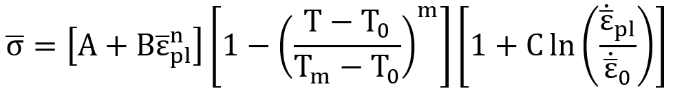
The dependence of the equivalent stress on the equivalent strain quantities, the equivalent plastic strain rate, and the temperature is well observed in this model, known as Johnson-Cook 1983. The mechanical response of a material to dynamic loads and the five constants A, B, n, C, and m are usually obtained from the results of a rod-to-wall impact test, which was performed for the first time in 1984 by Taylor.
Principle of Impulse and Momentum (Conservation Laws)
The total impulse acting on a body is equal to the change in momentum:
In a collision between two bodies (A and B), assuming no external forces, the total momentum is conserved:
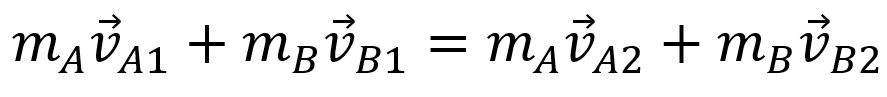
Where:
-
: initial velocities
-
: velocities after impact
Also, we have conservation law for:
- Angular Momentum: Conserved in systems with rotational motion and no external torques.
- Kinetic Energy: Only conserved in elastic impacts.
Types of Impact
Types of impact are categorized from different aspects. Two main aspects are velocity and energy behavior.
| Classification Type | Describes… | Related To… |
|---|---|---|
| Elastic/Inelastic | What happens to energy | Energy conservation & material response |
| High/Low/Hypervelocity | What happens due to speed | Kinetics, strain rate, damage behavior |
They are not conflicting — they just answer different questions.
Category by velocity
This is based on how fast the impact happens. Two primary types of impact velocity are low-velocity impact and high-velocity impact. Comparison of different types of impact are presented in the following table:
| Type | Speed Range | Energy Behavior | Description |
|---|---|---|---|
| Low-Velocity | < 10–50 m/s | Mostly elastic, low energy absorption | Objects deform slightly and return to shape; minimal permanent damage. Example: dropping a ball. |
| High-Velocity | 50 – 2000 m/s | Mostly inelastic, high-energy absorption | Significant deformation, fracture, or failure; much kinetic energy dissipated as heat, sound, and damage. Example: car crash. |
| Hypervelocity | > 2000 m/s | Near-complete inelastic; kinetic energy causes shock waves and material vaporization | Extreme energy release causing melting, vaporization, or fragmentation. Example: meteorite hitting Earth, bullet impact. |
This classification is about the dynamics of the impact: how fast, how violent, and what physics dominate (e.g., fluid-like behavior at hypervelocity).
Category by energy behavior
This is based on what happens to energy during the impact.
- Elastic Impact: All kinetic energy remains with the colliding bodies; objects bounce back without permanent change.
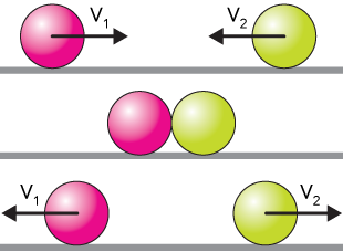
- Inelastic Impact: Some kinetic energy is lost to the surroundings in other forms (heat, deformation).
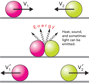
Figure 3: Inelastic Impact
- Perfectly Inelastic Impact: Maximum energy loss; two objects collide, stick together and move as one object thereafter.
| Type | What It Means | Based On |
|---|---|---|
| Elastic Impact | No kinetic energy lost (ideal case) | Energy conservation |
| Inelastic Impact | Some energy lost (sound, heat, deformation) | Partial energy loss |
| Perfectly Inelastic | Maximum energy loss, bodies stick together | Total energy loss |
This classification tells you how energy is transformed — like whether the objects bounce, deform, or stick.
Central Impact and Obilique Impact
The line of impact is a line through the mass centers of the colliding particles.
Central impact occurs when the directions of motion of the two colliding particles are along the line of impact.
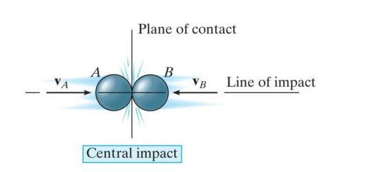
Figure 4: Central impact
Oblique impact occurs when the direction of motion of one or both of the particles is at an angle to the line of impact.
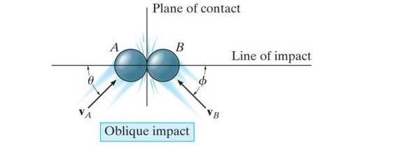
Figure 5: Oblique impact
What is Low Velocity Impact?
Low velocity impact refers to a collision where an object strikes a structure at relatively low speed, typically under 10 m/s. It is important in engineering because it can cause internal damage, delamination, or dents without visibly destroying the structure.
Common damage mechanisms (especially in composites)
In composites, low velocity impacts often cause matrix cracking, delamination, and Barely Visible Impact Damage (BVID). This hidden internal damage can seriously reduce residual strength even when the surface looks fine.
Typical metrics engineers track
- Peak force
- Absorbed energy
- Indentation depth
-
Residual strength from CAI (Compression After Impact) tests
What is High Velocity Impact?
High velocity impact occurs when an object strikes a target at speeds above about 10–1000 m/s. Such impacts generate significant stress waves, leading to penetration, fragmentation, or severe structural damage.
Typical speeds & ballistic considerations
High velocity impact usually means projectile speeds greater than 100 m/s. Contact time is extremely short, and inertial and stress-wave effects dominate. Aerospace debris, ballistic events, and defense scenarios are common examples.
(Image idea: Ballistic sequence frame captures. ALT text: “ballistic high velocity impact sequence”)
Damage modes
High velocity impacts lead to very different damage mechanisms compared to low velocity. Expect shear plugging, spalling, perforation, or even shock-induced failure depending on the projectile and target materials.
Measurement challenges
Because everything happens in microseconds, measurement requires high-speed cameras, chronographs, witness plates, and data acquisition at very high sampling rates.
The Importance of Impact Simulation
Simulating these events allows engineers to:
- Evaluate structural integrity and safety.
- Optimize material usage without compromising durability.
- Reduce the need for costly physical testing.
By capturing how a system responds to high-rate loading, engineers can predict failure modes, enhance product designs, and meet stringent safety standards.
Applications of impact dynamics (e.g., automotive, aerospace)
- Automotive: Crashworthiness assessments, pedestrian safety, bumper design.
Figure 6: Application of impact dynamics in automotive
- Aerospace: Bird strike analysis, runway debris impacts, satellite shielding.
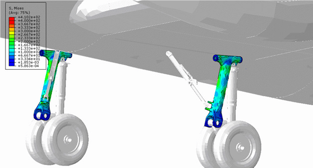
Figure 7: Application of impact dynamics in aerospace
- Consumer Electronics: Drop tests for mobile phones and laptops.
- Defense: Armor penetration, blast wave propagation.
- Sports Equipment: Helmet impact performance and protective gear design.
There is different software for simulating impact analysis, such as ABAQUS, ANSYS, COMSOL AND LSDYNA.
Abaqus Impact Simulation
Abaqus/Explicit is commonly used for Abaqus impact simulations due to its ability to handle short-duration, nonlinear events efficiently.
Part Definition
Create the geometry representing both the target and the impactor. Simplify complex features to reduce computational effort while retaining critical details.
Material Properties
Impact simulations require rate-dependent materials. Define:
- Density and elastic properties
- Plasticity models (e.g., Johnson-Cook for metals)
- Failure criteria, if fracture or damage is anticipated
Meshing Strategies
- Use fine mesh in high-stress or impact zones
- Prefer hexahedral elements (C3D8 or C3D8R) for accuracy
- Conduct mesh convergence studies to balance precision and runtime
Defining Boundary Conditions
- Apply realistic constraints matching physical supports
- Assign initial velocities or impact forces to the impactor
- Avoid over-constraining the model
An over-constraint means applying multiple consistent or inconsistent kinematic constraints. Many models have nodal degrees of freedom that are over-constrained. Such over-constraints may lead to inaccurate solutions or nonconvergence. Common examples of situations that may lead to over-constraints include (but are not limited to):
- contact slave nodes that are involved in boundary conditions or multi-point constraints;
- edges of surfaces involved in a surface-based tie constraint that are included in contact slave surfaces or have symmetry boundary conditions; and
- boundary conditions applied to nodes already involved in coupling or rigid body constraints.
Step Definition
- Use Dynamic Explicit step for transient impact events
- Define sufficient step duration to capture full response
- Adjust time increments automatically or manually for stability
Contact Definition
- Set surface-to-surface contact between impactor and target
- Include friction if necessary
- Tune contact stiffness and penalty parameters to avoid penetrations or instabilities
Common Challenges and How to Solve Them
Dealing with Convergence Issues:
- Use explicit dynamic solver to avoid typical implicit convergence problems
- Apply stabilization methods or reduce load increments in implicit runs
- Refine mesh and check for distorted elements
- Simplify contact and material models if needed
Managing Large Deformations and Contact Instabilities
- Use reduced integration elements with hourglass control (C3D8R)
- Adjust contact parameters to minimize penetration
- Consider adaptive meshing or remeshing strategies
- Use mass scaling cautiously to stabilize the simulation
Tips to Optimize Your Impact Simulation
Element Selection and Mesh Refinement can optimize impact simulation:
- Choose solid elements suitable for large deformation (C3D8R preferred)
- Refine mesh locally around impact zones
- Perform mesh sensitivity analysis for accuracy vs. cost tradeoff
Mass Scaling and Time Efficiency are also important:
- Apply mass scaling in low-strain regions to increase stable time increments
- Monitor energy balance to ensure physical accuracy
- Combine mass scaling with efficient step time controls to reduce computation time
Case Study: Low Velocity Impact
Low velocity impact refers to the collision between objects at relatively low speeds. While the impact energy may be lower compared to high-speed impacts, low-velocity impacts can still cause significant damage and deformation. Assessing the effects of low velocity impact is crucial for various industries to ensure the structural integrity, safety, and performance of their products.
For example, in the automotive industry, understanding the response of vehicles to low-velocity impacts is essential for designing crashworthy structures and improving occupant safety. In aerospace, assessing the impact resistance of aircraft components, such as fuselage panels or wings, helps ensure their ability to withstand ground handling incidents or bird strikes.
In this section, you will learn how to do low velocity impact simulations for the sandwich structure (corrugated aluminum core with two composite plates at the top and bottom) and subjected to the steel projectile.
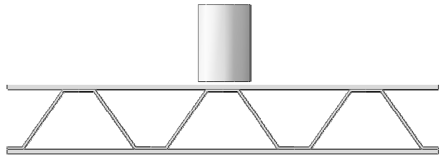
Figure 8: Configuration of corrugated sandwich structure
Core sandwich structures are produced using face sheets made of Epoxy-Glass fiber reinforced with aluminum alloy cores. This design concept allows sandwich structures to optimize their specific bending stiffness and strength while enhancing their ability to absorb energy.
To simulate the behavior of composites during impact, Hashin failure criteria has been employed. The explicit procedure is deemed suitable for this analysis, particularly when the sandwich panel experiences collapse during the impact.
Step 1: Modeling (Part Module)
To model corrugated core structure, perform the following steps:
Part→ Create→ 3D, Deformable, Shell, Extrusion, Continue
Also, the height of the cylinder must be entered equal to 0.115.
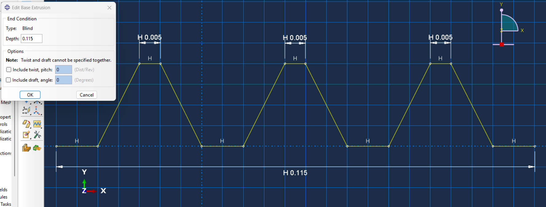
Figure 9: Sketching the part
The figure will be as follows:
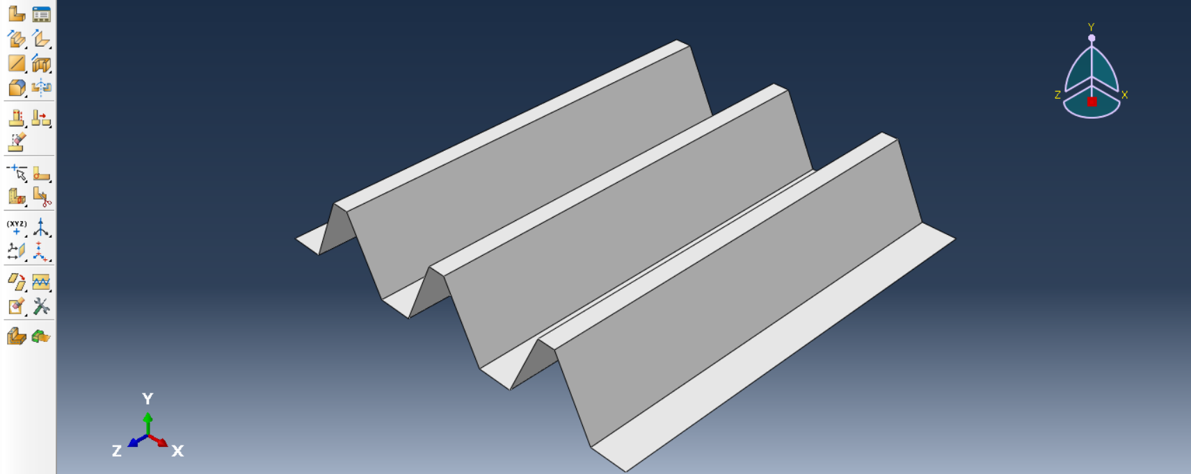
Figure 10: 3D model of corrugated plate
To model composite plate, use the following steps:
Part→ Create→ 3D, Deformable, Solid, Extrusion, Continue
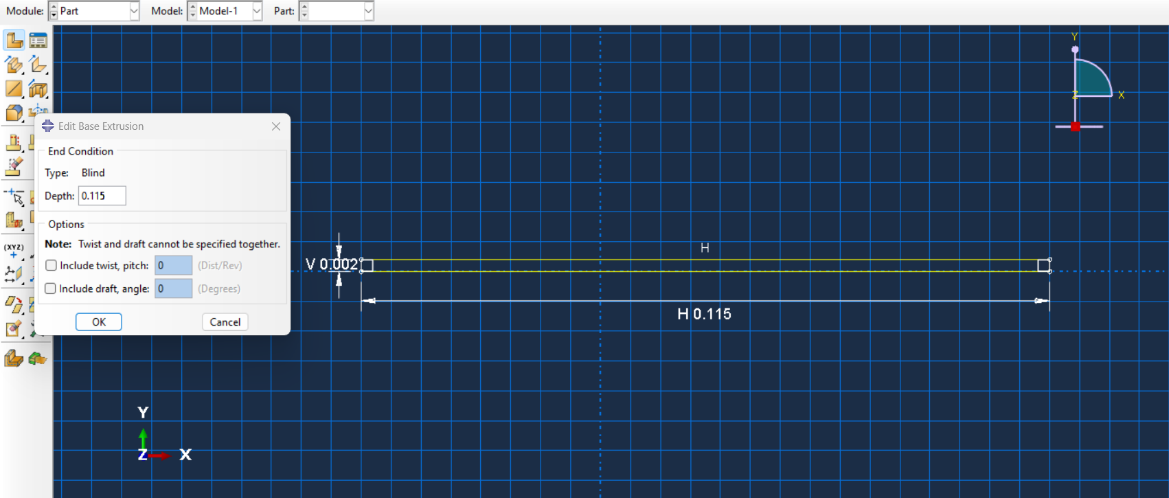
Figure 11: Sketching Composite Plate
The plate figure will be as follows:
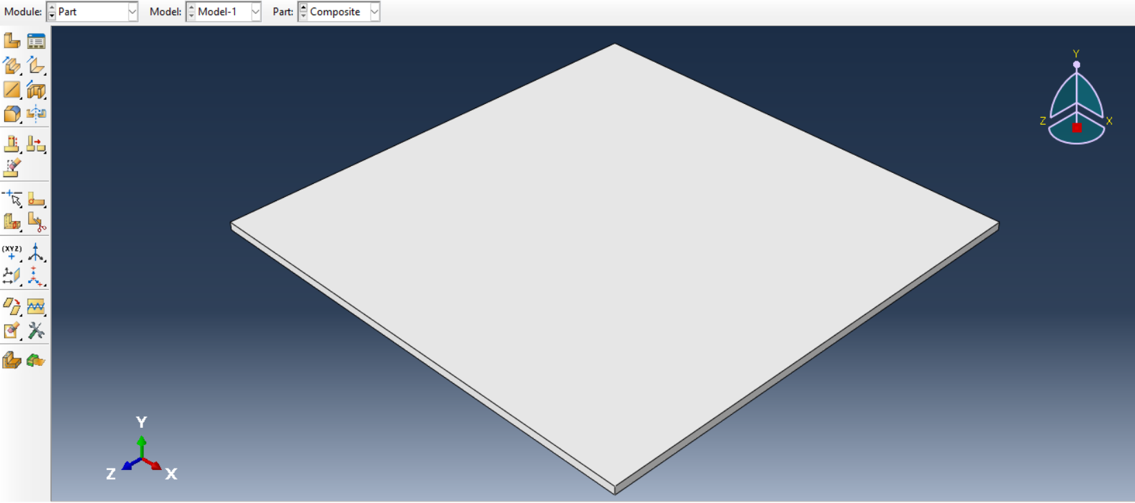
Figure 12: Composite Plate 3D model
To model projectile, use the following sketch.
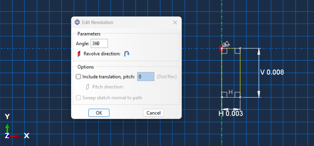
Figure 13: Sketching the projectile
Step 2: Mechanical properties (Property module)
To define the mechanical properties, we do the following:
Module: Property→ Material→ Create;
Material properties for corrugated plate: Mass density: 2760 (kg/m³), Young’s modulus: 70 (Gpa), Poisson’s ratio: 0.33.
The material parameters in the Johnson-Cook model must be defined in the data table, as shown below.
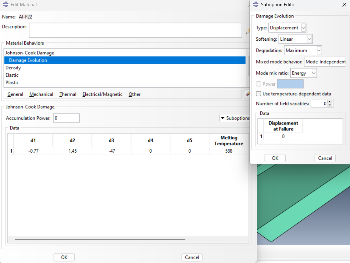
Figure 14: Johnson Cook Parameters
Also, plastic parameters are defined as shown below.
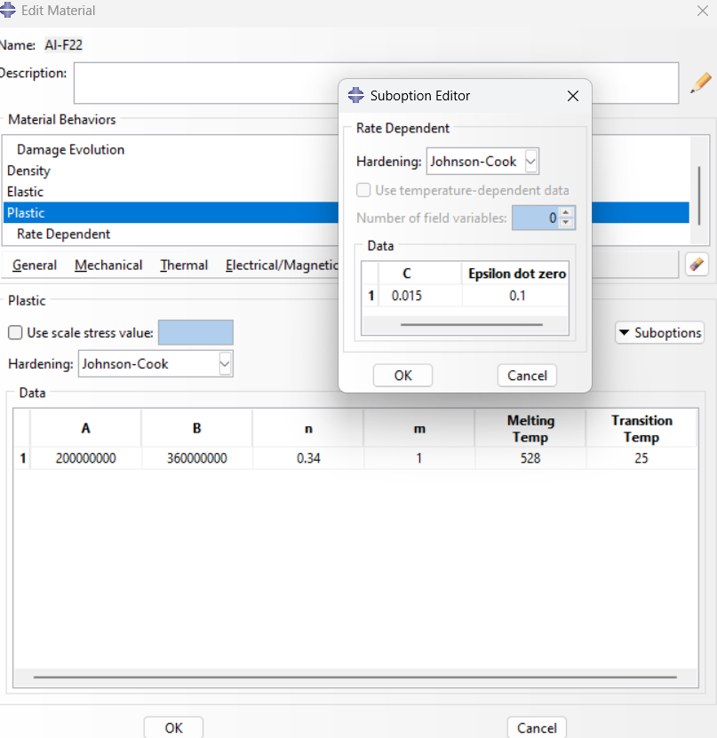
Figure 15: Plastic parameters
Material properties for composite plate: Mass density: 2200 (kg/m³), Young’s modulus: 210 (Gpa), Poisson’s ratio: 0.33.
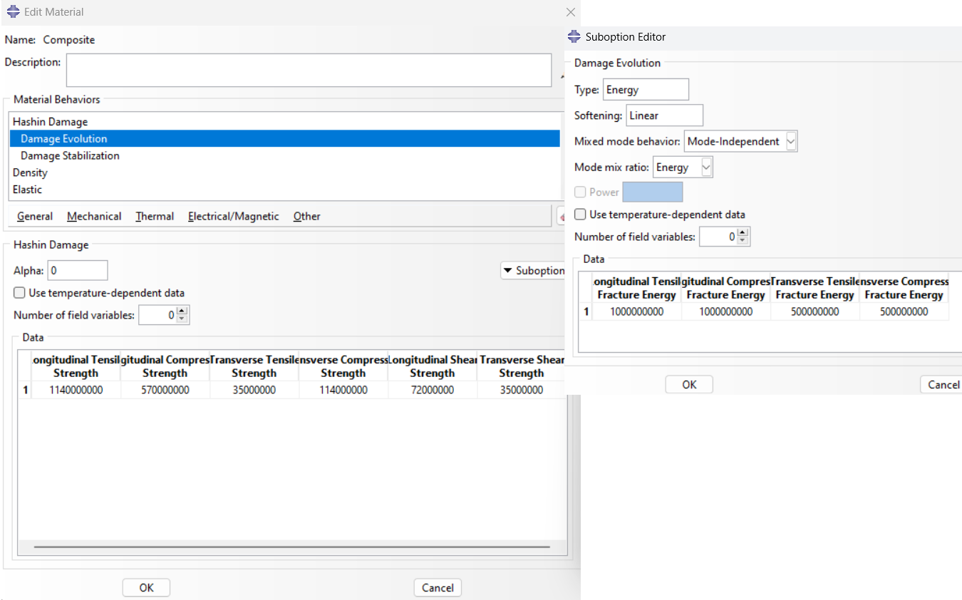
Figure 16: Hashin damage parameters for composite
Other parameters, such as damage stabilization are entered as follows:
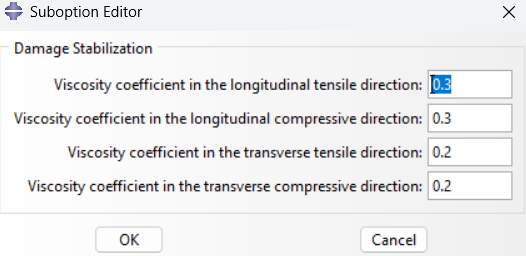
Figure 17: Hashin damage parameters for composite
Elastic parameters are defined as following:
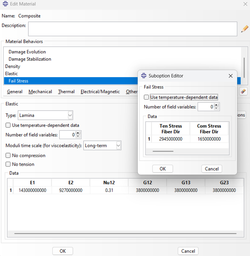
Figure 18: Elastic parameters
Also, define the rotation angle of composite layup.
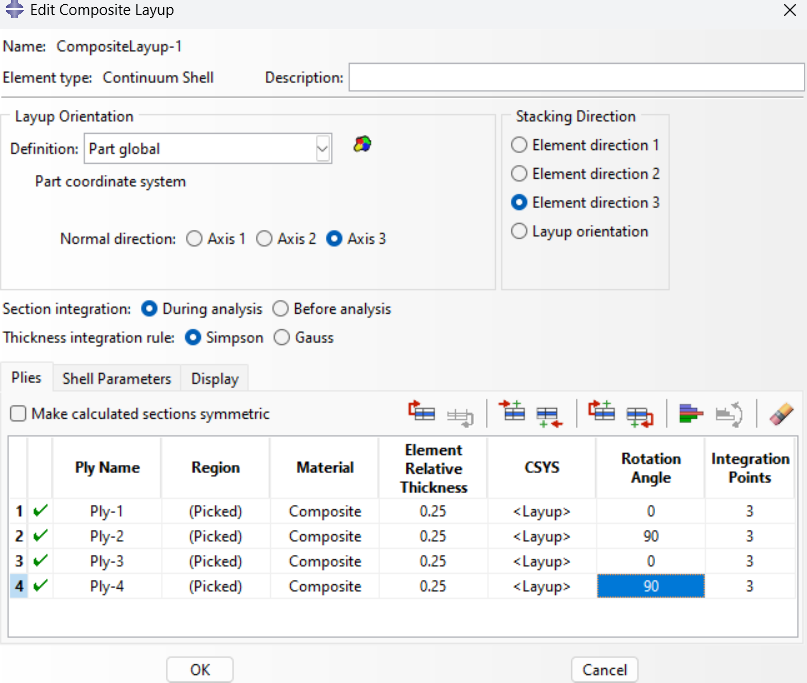
Figure 19: Composite layup
For projectile: Mass density: 7850 (kg/m³), Young’s modulus: 210 (Gpa), Poisson’s ratio: 0.33.
Other parameters, such as Expansion, Inelastic Heat Fraction and Specific Heat are entered as follows.
The material parameters in the Johnson-Cook model are specified, as shown below.
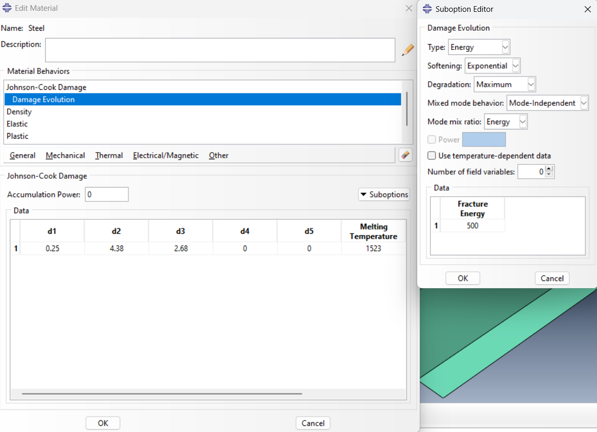
Figure 20: Damage parameters for projectile
Plastic rate dependent parameters are as this figure:
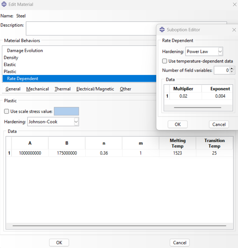
Figure 21: Plastic parameters for projectile
Step 3: Assembly module
Do the following to create an instance:
Module: Assembly→ Instance→ Create Instance; Instance Type: Independent→ OK
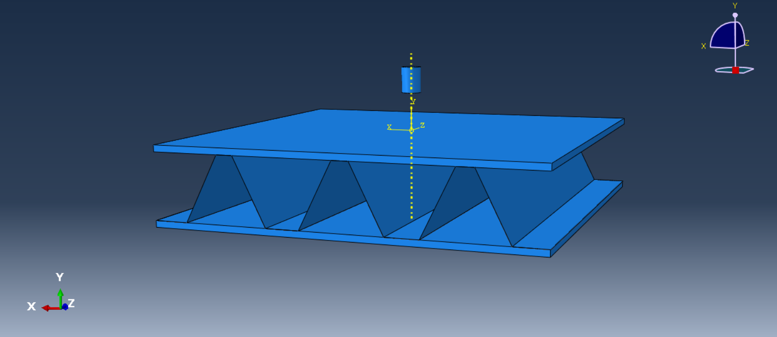
Figure 22: Assembled model
Step 4: Define the type of solution (Step module)
Module: Step→ Create Step; Procedure type: General; Dynamic, Explicit→ Continue
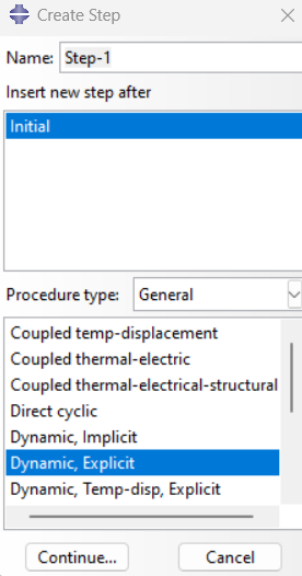
Figure 23: Selecting the step
Step 5: Boundary conditions (Load module)
The following method is used to define the boundary conditions and velocity of projectile:
Load Module: Create Boundary condition → Category→ Mechanical; Symmetry/Antisymmetry/Encastre→ Encastre;
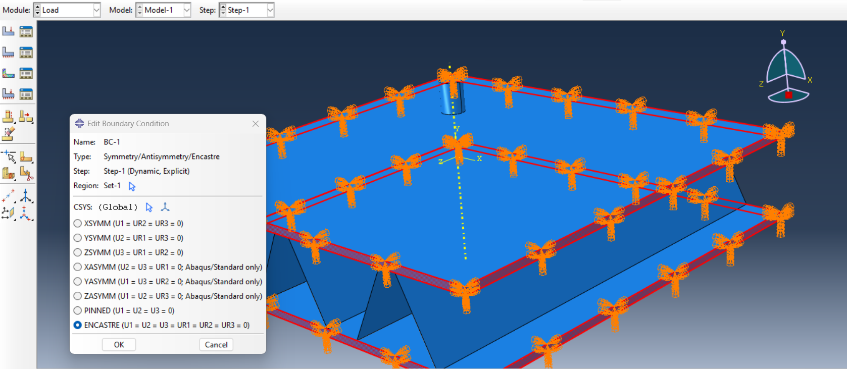
Figure 24: Defining Boundary condition
To define the initial impact velocity, do the following:
Load Module: Create Boundary condition → Category→ Mechanical; Velocity/Angular velocity;
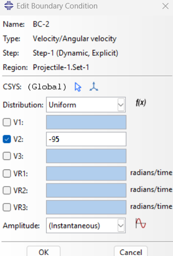
Figure 25: Defining velocity
Step 6: Meshing (Mesh module)
Mesh Module: Global seeds → Approximate global size: 0.001 →OK
Mesh Module: Assign Element Type→ Element Library: Explicit →Geometric Order: Linear→ Family: Continuum Shell
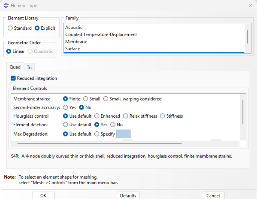
Figure 26: Assigning element type
Mesh Module: Mesh Part Instance→ Yes
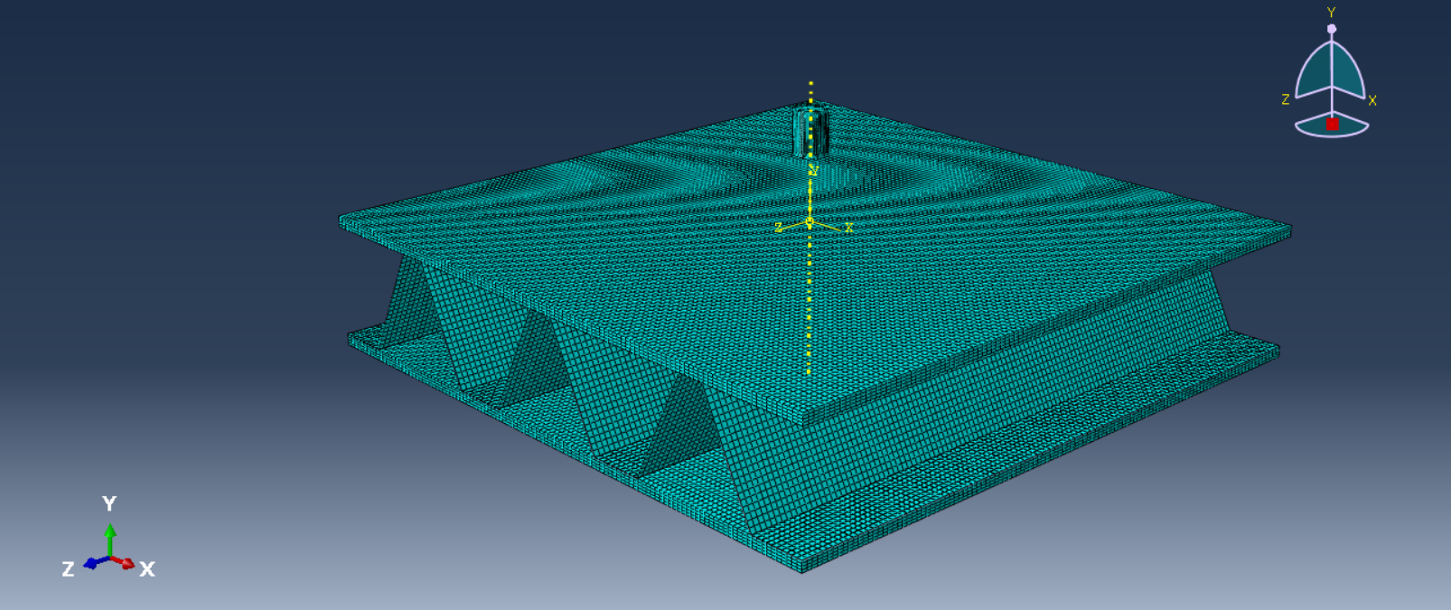
Figure 27: Meshed model
Step 7: Constraint and contact
You can use tie constraint between the core and composite plates.
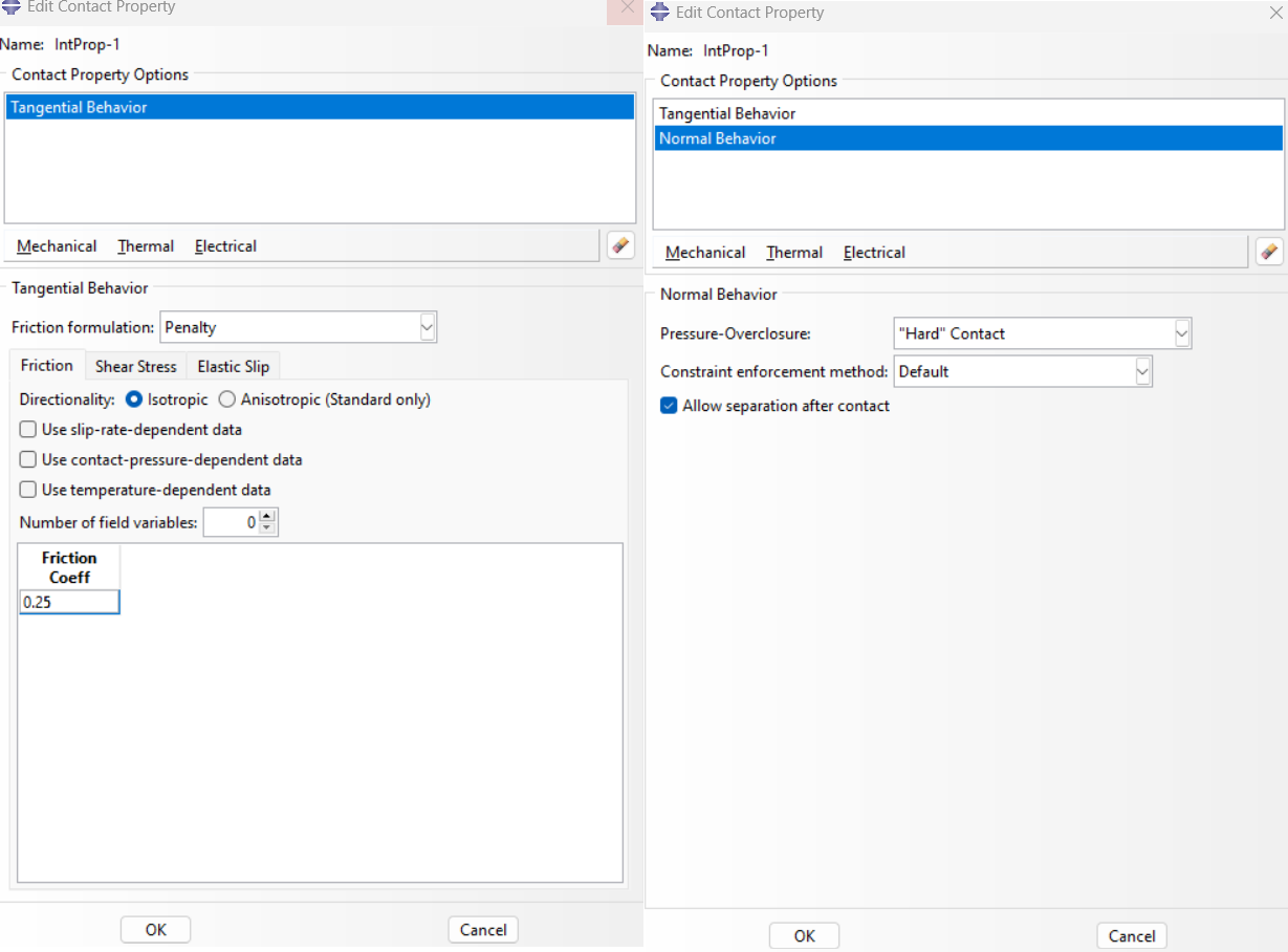
Figure 28: Defining Contact
Step 8: Solving problem (Job module)
Now the model is ready, follow the instructions below to analyze it.
Job Module: Create Job→ Continue…→ Edit Job → OK
The solution operation starts through the following path:
Job Module: Job Manager→ Submit
Step 9: Monitoring the Results (Visualization module)
The results can be viewed by the path below:
Job Module: Job Manager→ Results
Visualization Module: Plot→ Contours → On Deformed Shape
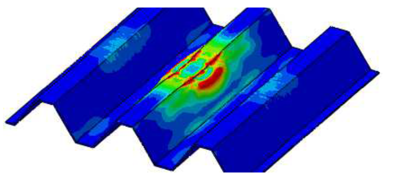
Figure 29: Results
High Velocity Impact Example
If you are interested in high velocity impact simulation tutorial, is available in this PDF file:
Conclusion
This article focused on the topic of impact dynamics, which refers to the short-duration collision between two bodies involving high force. It explained how impacts are studied in mechanical problems and why understanding them is important in real-world applications like vehicle crashes or drop tests.
The subject is important because impacts can cause significant damage or structural change, and engineers must predict and evaluate such events accurately. This helps in designing safer and more reliable products and systems.
The article began by defining impact and explained how impacts can be categorized based on velocity, duration, and object behavior. It introduced key concepts such as impulse, momentum, and the conservation of momentum, which are essential for analyzing impact problems. The next section discussed the difference between low- and high-velocity impacts, showing how each type affects objects differently. Finally, the article provided a basic guide to simulating impact in Abaqus, including the steps for setting up a model and how different velocities influence the simulation results.
Overall, this article gave a complete overview of impact dynamics by covering both theoretical concepts and practical simulation. It showed how impacts behave, how they are classified, and how engineers can analyze them using software tools like Abaqus.
Explore our comprehensive Abaqus tutorial page, featuring free PDF guides and detailed videos for all skill levels. Discover both free and premium packages, along with essential information to master Abaqus efficiently. Start your journey with our Abaqus tutorial now!