Simulating interactions between fluids and solids can be tricky, especially when materials undergo large deformations or impacts. Traditional methods often fall short when things start to move too much, stretch too far, or mix together. That’s where the Coupled Eulerian Lagrangian (CEL) method becomes useful.
The Coupled Eulerian Lagrangian method combines two different modeling strategies. One follows the material as it moves (Lagrangian), and the other keeps the mesh fixed while materials flow through it (Eulerian). Together, they allow engineers to simulate events like splashing, explosions, or objects hitting water without the problems of mesh distortion or complex setup.
In this article, we explain the basic ideas behind the Eulerian and Lagrangian approaches, then introduce the CEL method and how it works in Abaqus. We’ll cover key features like general contact, volume fraction, and material assignment. You’ll also see real examples where CEL is especially effective, and we’ll compare it with other methods like ALE, SPH, and CFD–FEA coupling. The goal is to help you understand when and how to use CEL for complex simulations.
Coupled Eulerian Lagrangian VS Eulerian VS Lagrangian
In finite element analysis (FEA), simulating real-world behavior often requires more than just capturing internal stress and strain. Many engineering problems involve complex interactions between solids and fluids, high-speed impacts, or materials undergoing large deformations. Traditional mesh-based approaches can struggle under such conditions. This is where the Coupled Eulerian Lagrangian (CEL) method becomes invaluable.
To appreciate the power and purpose of the coupled Eulerian Lagrangian method, it’s helpful to first understand the two fundamental frameworks it merges the Eulerian approach and the Lagrangian approach. These two methods define how material motion is handled during a simulation, and each has its own strengths and limitations.
Before we explore them in detail, the table below gives a quick overview to help clarify their key differences:
| Feature / Method | Eulerian | Lagrangian | Coupled Eulerian–Lagrangian (CEL) |
|---|---|---|---|
| Mesh Behavior | Fixed in space | Moves with material | Combination: Eulerian mesh for fluids, Lagrangian for solids |
| Ideal For | Fluids, gases, soft materials with large flow |
Solids, structural components |
Fluid–structure interaction, large deformation problems |
| Handles Large Deformation? |
Yes (fluid flow) | No (mesh distortion occurs) | Yes (fluid and structure can interact robustly) |
| Material Tracking | Volume fraction in each element | Material is tracked by mesh nodes |
Both: Eulerian for fluid, Lagrangian for structure |
| Typical Use Cases | Slashing, blast waves | Plastic deformation, stress analysis |
Ball hitting water, fuel tank under blast, soil impact |
Now let’s break Eulerian, lagrangian and Coupled Eulerian Lagrangian approaches down.
Eulerian Approach
In the Eulerian formulation, the computational mesh remains fixed in space, and the material flows through it. This is the standard approach in computational fluid dynamics (CFD). The solver tracks how materials move across the elements rather than how the mesh itself deforms. A useful analogy is to imagine a stationary camera watching a river: the camera doesn’t move, but the water flows past the lens.
The Eulerian approach is ideal for modeling fluids, gases, molten materials, or bulk deformable such as sand or soil, where the material motion and deformation is severe.
However, while the Eulerian method is excellent for capturing flow, it is not suitable for tracking the deformation of solid structures. That is where the Lagrangian method comes in.
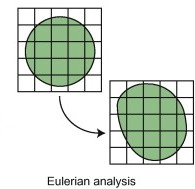
Figure 1: schematic of eulerian approach meshing [Ref]
Lagrangian Approach
The Lagrangian formulation, in contrast, involves a mesh that follows the material motion. Each node in the mesh moves with the material it represents. This is the standard approach for solid mechanics and structural simulations. Imagine placing a camera on a boat floating down a river. It moves along with the flow, capturing the changes in the environment around it. In simulation terms, this means that the material coordinates are fixed relative to the mesh.
The Lagrangian method is best suited for modeling solids, such as metals, polymers, or structural components. It provides high accuracy for capturing local deformations, stress concentrations, plasticity, and failure. However, one of its main limitations is mesh distortion under extreme deformations.
When a solid experiences very large strains such as tearing, folding, or impacting a fluid surface, the mesh elements can become severely distorted, leading to poor accuracy or simulation failure.
This limitation becomes critical in simulations where fluid structure interaction (FSI), penetration, or large displacement impacts are involved. In such cases, a single formulation is not sufficient, and a more advanced method is needed.
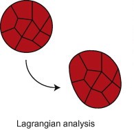
Figure 2: Schematic of lagrangian approach meshing [Ref]
What is Coupled Eulerian Lagrangian Method?
In many engineering simulations—especially those involving fluids or soft materials—traditional modeling methods begin to break down when deformation becomes extreme.
The Lagrangian method is commonly used for solid structures. It assumes the mesh moves with the material, which works well for moderate deformations. However, under severe distortion—such as high-speed impact, large-scale flow, or violent structural interaction—the mesh can stretch too far. This leads to accuracy issues or even causes the simulation to fail.
On the other hand, the Eulerian method uses a fixed mesh. It handles large deformations and fluid motion well. But it struggles to model solid structures or their mechanical behavior accurately under load.
The Limitations of Single-Method Approaches
This creates a significant limitation. Many real-world problems involve both fluid-like motion and solid structural behavior at the same time. These elements interact closely and influence each other.
Using only one method—Eulerian or Lagrangian—often oversimplifies the physics. It can miss critical interactions, making the results less reliable.
The Solution: Coupled Eulerian Lagrangian Method
This is where the coupled Eulerian Lagrangian (CEL) method becomes essential. It bridges the gap by combining the strengths of both approaches:
-
Solids are modeled using a Lagrangian mesh. This captures structural deformation and internal stresses with high accuracy.
-
Fluids or highly deformable materials use a stationary Eulerian mesh. This allows them to flow or splash freely without distorting the mesh.
Most importantly, the interaction at the interface—where solids and fluids meet—is handled automatically. The entire simulation runs smoothly within the same environment.
Why Engineers Choose CEL in Abaqus
Engineers are not selecting CEL just because it’s advanced. They rely on it because traditional methods can’t handle the full complexity of the problems they face.
Whether it’s:
-
Fluid motion inside a container,
-
Impact into soft ground, or
-
Fluid-structure interaction under dynamic conditions,
The CEL method provides a stable, accurate, and physically realistic solution.
It enables a unified simulation that captures both material flow and solid response. This makes CEL in Abaqus a powerful tool for advanced nonlinear analysis.
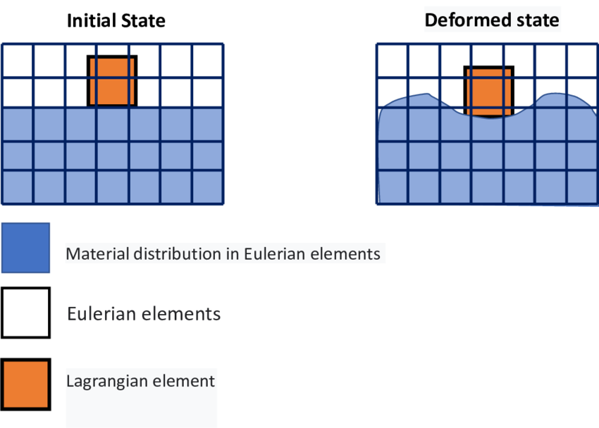
Figure 3: Schematic of coupled eulerian-lagrangian approach meshing [Ref]
Abaqus Coupled Eulerian Lagrangian
The coupled Eulerian Lagrangian method becomes especially powerful when implemented within Abaqus/Explicit. Unlike many simulation platforms that require third-party solvers or external tools, Abaqus provides a fully integrated CEL framework that supports both the definition and interaction of Eulerian and Lagrangian domains in a single environment.
This capability allows engineers to simulate fluid–structure interaction, material mixing, and large deformation problems with greater efficiency and control.
Within coupled Eulerian Lagrangian Abaqus models, both fluid and structural parts can be built, meshed, and assigned appropriate behaviors entirely inside Abaqus/CAE. There’s no need for external CFD packages or co-simulation setups. Everything — from mesh generation to contact definition and post-processing — is handled within the same interface.
What makes the CEL implementation in Abaqus particularly flexible is its ability to handle multiphase flows, free surfaces, and complex geometries using a fixed Eulerian mesh. Material flow is controlled and tracked using Eulerian Volume Fraction (EVF) values, allowing materials to move freely through the Eulerian mesh while interacting with solid structures.
These interactions are managed automatically using General Contact, removing the need to manually define contact pairs between domains.
Generally, there is no built-in option to use the CEL method in Abaqus software, but users can benefit from this method by making some settings. In the next steps, we will address the parts of the simulation process using the CEL method that users have the most problems and errors in using.
Part Type
The most basic part of using the CEL method is to create a suitable model for the fluid component of the simulation. Don’t forget that use CEL, an Eulerian part must be created.
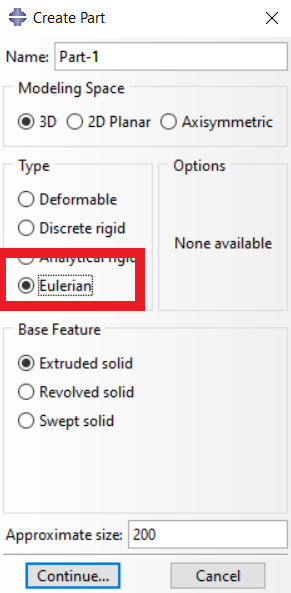
Figure 4: Create part as an Eulerian part
Material Property
Material definition in CEL models requires two parts:
Eulerian Materials: These typically represent fluids or soft media. In Abaqus, they are assigned using the Equation of State (EOS) property. This defines the pressure–density relationship and is crucial for simulating compressibility, shock behavior, and cavitation. Common EOS models include Ideal Gas, and Us-Up relations. Advanced behaviors like viscous flow or non-Newtonian fluids require user subroutines like VUVISCOSITY.
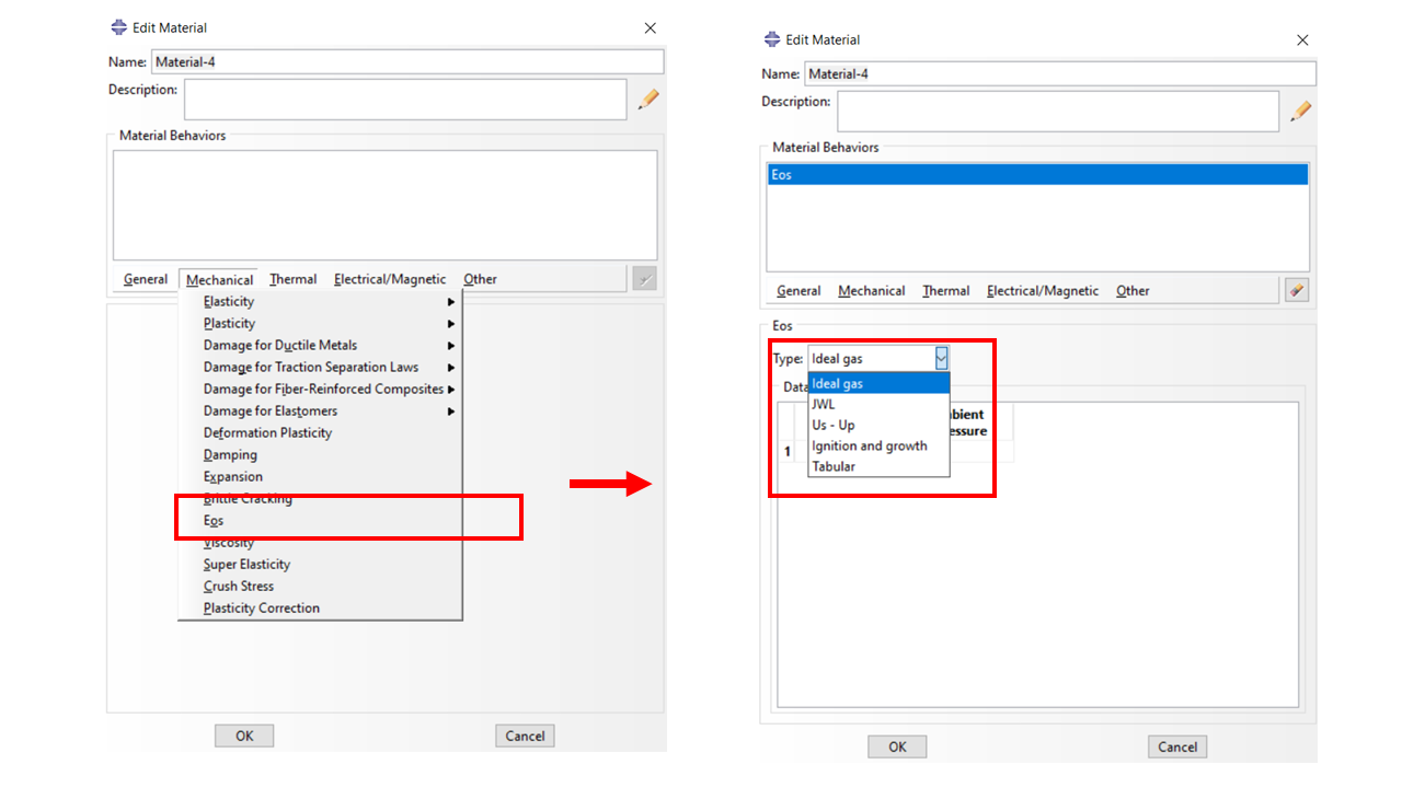
Figure 5: EOS material property in Abaqus
Lagrangian Materials: These are assigned to solid parts. They follow standard material models such as linear elasticity, plasticity, or hyperelasticity.
Dynamic Explicit Step
All coupled Eulerian Lagrangian simulations in Abaqus are run using the Explicit Dynamics procedure. This solver is designed for problems involving:
- High strain rates
- Transient dynamic loading
- Large deformations
For CEL, where Eulerian meshes are usually fine, time increments are very small. This leads to high computational cost, but also ensures stability and accuracy for nonlinear behavior.
Defining Contact Between Parts
In traditional contact modeling, users need to define specific contact pairs. But in coupled Eulerian Lagrangian Abaqus models, contact is handled automatically through General Contact. This algorithm detects interactions between the Eulerian domain (fluid) and the Lagrangian domain (structure) without requiring manual setup of contact surfaces.
The core idea is based on immersed boundary contact. As the Lagrangian body moves into the Eulerian region, it displaces the fluid. Abaqus calculates this interaction using volume fraction, checking whether a given Eulerian element is filled and whether it overlaps with a solid structure. This allows accurate transfer of momentum, pressure, and contact force.
- General Contact supports:
- Contact between multiple structures and multiple fluids
- Self-contact in highly deformable materials
- Automatic contact enforcement without stabilization parameters
This feature is one of the reasons why CEL in Abaqus is much easier to implement compared to other ways.
Material Assignment & Volume Fraction
The Eulerian Volume Fraction (EVF) is a critical concept in CEL. It represents the percentage of an Eulerian element that is filled with material. For example, a volume fraction of 1.0 means the element is completely filled, while 0.0 means it’s empty. This value changes dynamically as material flows through the mesh.
In multiphase simulations, each material is tracked separately using a unique EVF variable. This enables modeling of interfaces between materials such as water–air surfaces, or molten-solid boundaries without special meshing or contact definitions.
In Abaqus/CAE, volume fraction is initialized through Predefined Fields, material assignment. You define which regions contain which materials at the start of the simulation. During the analysis, these fields evolve naturally based on flow and interaction.
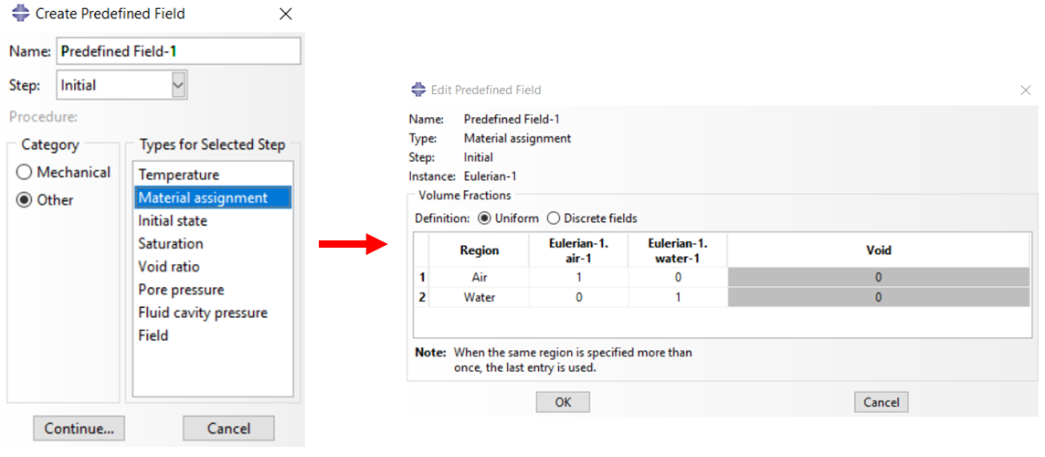
Figure 6: volume fraction for water–air surfaces
Meshing
The last step of modeling and using the CEL method is meshing and appropriate element selection. Considering that the problems solved using the CEL method are very time-consuming, the use of partitioning and selecting the appropriate size of the elements is very effective in saving the time. On the other hand, for Eulerian section, the Eulerian element family must be used, which is available by default in Abaqus.
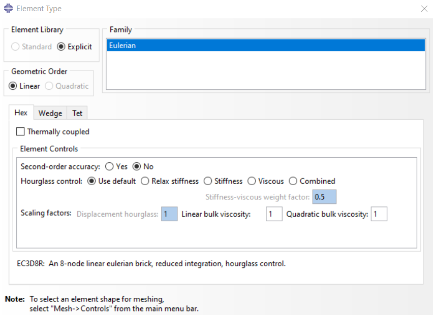
Figure 7: Selecting Eulerian element for Eulerian material
Coupled Eulerian Lagrangian (CEL) analysis: Some Examples
Below are common engineering problems where the coupled Eulerian Lagrangian method provides unique advantages:
- Liquid Storage Tank Under Blast: Model structural deformation of the tank, as well as internal fluid surge and pressure rise.
- Water Impact Simulation: For example, a flow of water hitting a dam.
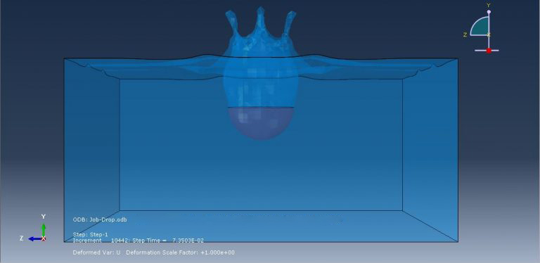
Figure 8: Projectile impact on water (get the full tutorial of this example and its file through here)
- Soil Impact: Penetration of projectiles or tools into granular soil, avoiding mesh distortion typical in Lagrangian-only methods. You can learn more about soil analysis in Abaqus in our latest blog: “Abaqus Soil Modeling | Key Models and Applications“.
- Ball Impact on Water: A benchmark fluid–structure interaction case, often used in validating simulation tools.
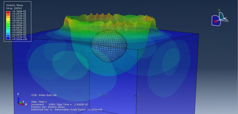
Figure 9: Ball impact on the water (get the full tutorial of this example and its file through here)
CEL Against Other Approaches: Comparisons
While the coupled Eulerian Lagrangian method in Abaqus is a powerful and flexible tool, it is not the only approach available for problems involving large deformations and fluid–structure interaction (FSI). Depending on the type of simulation, engineers may also consider methods like ALE (Arbitrary Lagrangian–Eulerian), SPH (Smoothed Particle Hydrodynamics), or CFD–FEA co-simulation.
Each method has its advantages and limitations. In this section, we compare the coupled Eulerian Lagrangian Abaqus approach with its alternatives, so that you can understand when CEL is the best choice and when it’s not.
- ALE (Arbitrary Lagrangian Eulerian)
The Arbitrary Lagrangian–Eulerian (ALE) method blends the Lagrangian and Eulerian approaches by allowing the mesh to move independently of the material, offering moderate flexibility and reduced mesh distortion.
It’s effective for simulations involving moderate deformation, such as metal forming or soft-body indentation, and supports mesh smoothing and remeshing in Abaqus/Explicit. However, ALE becomes less reliable under extreme deformation, where frequent remeshing can complicate the analysis and reduce accuracy.
It also lacks built-in support for multiphase flow and volume fraction tracking, making it less suitable than the coupled Eulerian Lagrangian method for complex fluid–structure interaction problems.
- SPH (Smoothed Particle Hydrodynamics)
Smoothed Particle Hydrodynamics (SPH) is a mesh-free method where materials are represented by particles. It excels in modeling fragmentation, splashing, and extreme deformation without mesh distortion. However, SPH is computationally demanding, less accurate for pressure-based problems, and sensitive to parameter settings. Unlike the coupled Eulerian Lagrangian method, it lacks volume tracking and strong coupling with structural elements.
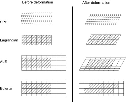
Figure 10: Mesh schematic of CEL, AEL, and SPH methods
- CFD–FEA Coupling
CFD–FEA co-simulation uses separate solvers for fluid and structure, exchanging data at each time step. It enables high-fidelity fluid modeling (e.g., turbulence, heat transfer, multiphase flow) and is widely used in aerospace, biomechanics, and automotive applications. However, it involves complex setup, interface management, and solver synchronization, making it less suitable for fast or deformation-driven problems.
In contrast, the coupled Eulerian–Lagrangian method in Abaqus offers a more streamlined, single-solver solution for such cases.
| Feature / Method | CEL | ALE | SPH |
|---|---|---|---|
| Mesh Type | Fixed mesh for fluids (Eulerian), moving mesh for solids (Lagrangian) | Mesh moves independently from material | Meshless (particles) |
| Mesh Distortion Risk | None for Eulerian, low for Lagrangian | Reduced but not eliminated | None |
| Ideal For | FSI with large deformation, impact, splashing | Moderate deformation, forming, soft-body contact | Fragmentation, erosion, splash, free surfaces |
| Multiphase / Volume Tracking | Yes (via Volume Fraction in Eulerian elements) | Limited | No |
| Coupling Between Fluids and Solids | Native and automatic inside Abaqus | Manual or partial | Weak (requires special treatment) |
| Computational Cost | High (due to fine mesh and small time steps) | Moderate | Very high |
| Accuracy in Pressure Fields | High for FSI and structural response | Moderate | Often lower |
| Use Cases | Ball–water impact, blast in fluid-filled tank, soil penetration | Metal forming, balloon expansion, tube collapse | Explosion, splash, granular breakup |
| Implemented in Abaqus | Yes (Abaqus/Explicit only) | Yes (mainly Abaqus/Explicit) | Yes (via SPH elements) |
Conclusion
This article introduced the Coupled Eulerian Lagrangian (CEL) method, a simulation approach that combines both Eulerian and Lagrangian formulations to handle problems involving large deformations and fluid–structure interaction. It is especially useful when traditional methods face limitations due to mesh distortion or complex material behavior.
We first explained the basics of the Eulerian and Lagrangian approaches, then showed how CEL integrates them to simulate challenging scenarios like impact, splashing, or internal explosions. The article also covered how Abaqus supports CEL through features like General Contact, Volume Fraction, and Material Assignment. Several practical examples were presented to highlight typical CEL use cases.
Finally, we compared CEL with alternative methods such as ALE, SPH, and CFD–FEA co-simulation to help clarify where CEL fits best. In summary, CEL in Abaqus offers a balanced solution for simulating complex interactions between fluids and solids in one environment.
Explore our comprehensive Abaqus tutorial page, featuring free PDF guides and detailed videos for all skill levels. Discover both free and premium packages, along with essential information to master Abaqus efficiently. Start your journey with our Abaqus tutorial now!