Abaqus Soil Modeling | Key Models and Applications

Do you think understanding soil behavior is easy?! Soil doesn’t act like a solid rock—it moves, settles, expands, and even turns to liquid during earthquakes. These behaviors make predicting soil response one of the most complex challenges in civil and geotechnical engineering. Understanding how soil reacts under various forces is key to building safe foundations, bridges, tunnels, and more.

In geotechnical engineering, Abaqus geotechnical modeling is widely used to simulate soil behavior, soil–structure interaction, and subsurface engineering problems. Abaqus provides advanced constitutive soil models and numerical tools that make it a powerful platform for geotechnical analyses such as foundation design, slope stability, consolidation, and seismic soil response.

To handle these challenges, engineers often use simulation tools like Abaqus. This software helps analyze soil behavior under stress, seismic loading, and interaction with structures. Abaqus includes a wide range of material models and features, such as Mohr-Coulomb, Drucker-Prager, and advanced clay models, as well as powerful methods like the Coupled Eulerian–Lagrangian (CEL) approach for large deformation analysis.

In this article, we explain how Abaqus can be used to simulate different soil behaviors and structural interactions. We’ll look at the most common Abaqus soil models available in the software, their features, and when to use them. If you’re working in geotechnical or structural engineering, this guide gives you a clear overview of how to Abaqus soil modeling effectively.

Introduction to Abaqus soil modeling

Abaqus is a powerful finite element analysis (FEA) software widely used in geotechnical engineering to simulate complex soil behaviors and soil-structure interactions. Abaqus Soil Modeling capabilities allow engineers to model various scenarios with high accuracy, leading to better-informed design decisions.

Soil-structure Interaction (SSI) refers to the mutual response between a structure and the supporting soil when subjected to loads, especially dynamic or seismic ones. Unlike rigid foundations, real-world foundations and their underlying soils deform under stress. This interaction plays a critical role in the accuracy of simulations and the reliability of engineering designs.

Here are the key points:

• Importance in Realistic Modelling: Traditional designs often assume a fixed or rigid base. However, this ignores the actual behavior of soil, which can deform, consolidate, or even fail under loading. By including SSI, engineers achieve more realistic predictions of structural response, especially for buildings, bridges, tunnels, retaining walls, and offshore structures.
• Dynamic Loading Sensitivity: In seismic engineering or vibration analysis, SSI significantly influences the system’s natural frequency and damping. Neglecting it can underestimate displacements or overdesign the foundation system.
• Foundation Design Optimization: Understanding SSI helps optimize foundation size and type (shallow, deep, pile, mat) and improves the overall efficiency of structural design by accounting for how loads are distributed into the soil.
• Soil Nonlinearity and Heterogeneity: Soils exhibit complex behaviors such as plasticity, anisotropy, strain-rate dependency, and pore pressure effects. These characteristics must be considered in advanced simulations that are directly related to soil structure interaction—something Abaqus is well-equipped to handle.

Figure 1: Example of dynamic loading simulation (earthquake) on dam and soil

You can find the complete example in the figure above in this tutorial: Workshop-13: Earthquake over gravity dam in interaction with water and soil using Abaqus

Abaqus uses powerful tools that can make this software superior in soil analysis. These advantages include:

• Advanced Material Models: Abaqus offers a range of constitutive models to represent different soil types and behaviors accurately.
• Coupled Analyses: The software can perform coupled pore pressure-stress analyses, essential for evaluating consolidation and liquefaction phenomena.
• Dynamic Loading Simulations: Abaqus can simulate the impact of dynamic loads, such as earthquakes, on soil and structures.
• Customization: Users can implement custom material models and subroutines to tailor analyses to specific their needs.

Soil behavior in eyes of engineers

Soil behavior encompasses the study of how soil materials respond to various physical, mechanical, and environmental conditions. This includes analyzing properties such as strength, compressibility, permeability, and stress-strain relationships. Soil behavior is influenced by factors like moisture content, density, mineral composition, and loading conditions.

Examples of Concepts and phenomena that are important in studying soil behavior:

• Shear Strength: The resistance of soil to shear stress is crucial in determining slope stability and bearing capacity.
• Consolidation: Over time, saturated soils may compress under load, leading to settlement—a critical consideration in foundation design.
• Liquefaction: During seismic events, saturated sandy soils can lose strength and stiffness, behaving like a liquid, which poses significant risks to structures. Like when you wiggle your toes in the wet sand near the water at the beach. This effect can be caused by earthquake shaking.
• Swelling and Shrinkage: Clays can expand or contract with moisture changes, affecting the integrity of pavements and foundations.

Understanding these behaviors is essential for geotechnical engineers to design safe and effective structures.

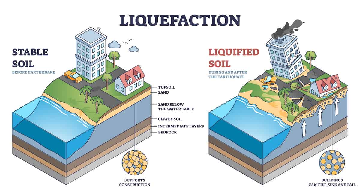
Figure 2: Understanding soil liquefaction

In geotechnical engineering, accurate representation of soil behavior is essential for reliable design. Abaqus geotechnical modeling allows engineers to incorporate stress history, confinement effects, and drainage conditions into numerical simulations for geotechnical applications.

Overview of Abaqus Soil Models and Their Capabilities

Abaqus offers several ways to simulate the complex behavior of soils under various loading conditions. These Abaqus soil models are essential for accurately predicting soil responses in geotechnical engineering applications.

Mohr-Coulomb Model

The Mohr-Coulomb model is a classical elastoplastic model used to describe the shear strength of soils and rocks. It is defined by two parameters: cohesion (c) and internal friction angle (φ). This model is particularly suitable for simulating the behavior of granular materials like sand and gravel under shear stress. The Mohr-Coulomb yield criterion is expressed as:

Where:

•  is the shear stress
• C is cohesion
•  is normal stress on the failure plane
•  is the angle of internal friction

In terms of principal stresses, the criterion can be represented as:

In Abaqus soil modeling, the Mohr-Coulomb model is implemented as an elastoplastic material model with a yield function based on the Mohr-Coulomb criterion. This model is available from the mechanical, Plasticity menu.

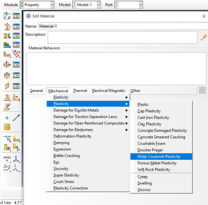
Figure 3: Selecting Mohr-coulomb model in Abaqus

It includes isotropic cohesion hardening/softening and allows for the definition of tension and compression cutoffs. The model can be used in both Abaqus/Standard and Abaqus/Explicit analyses.

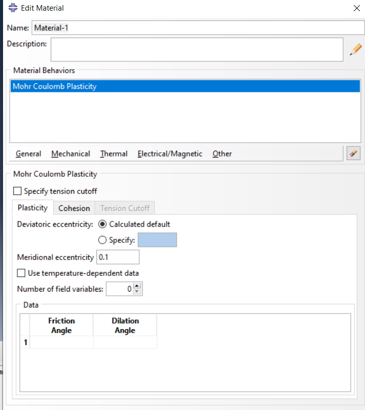
Figure 4: Mohr-Coulomb model in Abaqus

Clay Plasticity Model

The Clay Plasticity model in Abaqus soil modeling is designed to capture the complex behavior of cohesive soils, particularly clays, under different stress states. It is grounded in critical state soil mechanics and is suitable for modeling the elastoplastic behavior of normally consolidated and lightly overconsolidated clays. This model is particularly effective for simulating scenarios such as embankment construction, excavation, and foundation loading, where accurate prediction of soil deformation and failure is crucial.

The yield surface in the Clay Plasticity model is defined in terms of the mean effective stress p, deviatoric stress q, and pre-consolidation pressure p_c​:

Where:

• q is deviatoric stress.
• P is mean effective stress.
• p_c is pre-consolidation pressure.
• M is the slope of the critical state line in the p-q plane.

This equation represents an elliptical yield surface in the p-q space, capturing the pressure-dependent yielding behavior of clays.

In Abaqus soil modeling, the Clay Plasticity model is implemented in the Plasticity menu. This model is available in both Abaqus/Standard and Abaqus/Explicit.

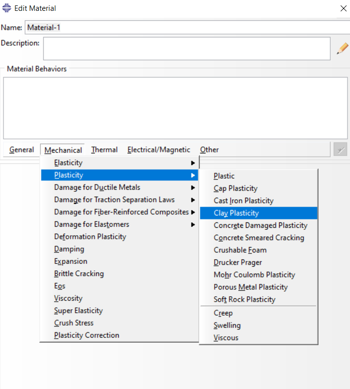
Figure 5: Selecting clay plasticity model in Abaqus

When users select this model in Abaqus there are some parameters that they must define. They include:

• Logarithmic Plastic Bulk Modulus: Defines the compressibility of the soil.
• Stress Ratio at Critical State: Determines the shape of the yield surface.
• Initial Yield Surface Size: Specifies the initial size of the yield surface.
• Wet Yield Surface Size: Defines the size of the yield surface on the “wet” side of the critical state.
• Flow stress ratio: Ratio of the flow stress in triaxial tension to that in triaxial compression.

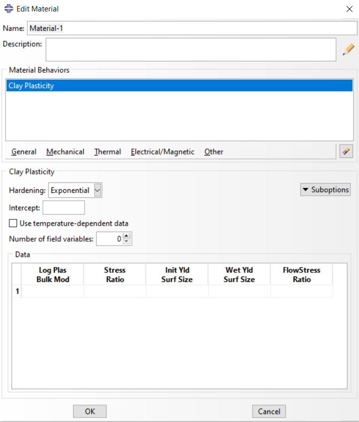
Figure 6: Clay Plasticity model sub-menu in Abaqus property module

Drucker-Prager Model

This model is a pressure-dependent plasticity model often used in geotechnical simulations as an alternative to the Mohr-Coulomb model. It offers a smooth yield surface, which enhances numerical stability and convergence in finite element simulations, especially under complex loading conditions. The yield criterion for the Drucker-Prager model is defined by this equation:

Where:

• q is deviatoric stress.
• p is mean stress.
• β is the friction angle.
• d is the cohesion parameter.

This smooth, conical yield surface makes the model particularly well-suited for modeling materials like soils and rocks that exhibit pressure-sensitive behavior. Due to its robust and mathematically convenient formulation, it is widely used in applications involving slope stability, foundation behavior, and underground excavations where accurate stress predictions and stable solutions are essential.

Abaqus includes the Drucker-Prager model with options for perfect plasticity or isotropic hardening. Users can define parameters such as the friction angle, cohesion, and dilation angle. The model is applicable in both Abaqus/Standard and Abaqus/Explicit analyses.

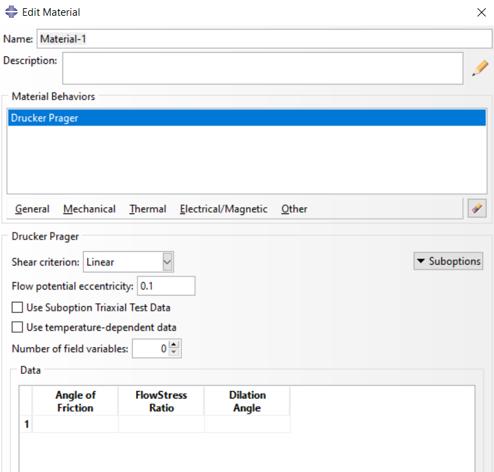
Figure 7: Drucker-Prager model in Abaqus

Cap Plasticity Model

The Cap Plasticity model is used to simulate materials that exhibit pressure-dependent yielding with hardening behavior, such as soils, rocks, and concrete. It combines a Drucker-Prager-type shear failure surface with a cap to model compaction behavior under high hydrostatic pressures.

The yield surface consists of a shear failure surface and a cap yield surface. The cap yield surface is typically defined as:

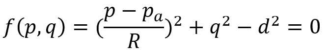
Where:

• p is the hydrostatic pressure,
• q is the deviatoric stress,
• p_a​ is the cap position,
• R is the cap eccentricity,
• d defines the size of the yield surface.

In Abaqus, the Cap Plasticity model requires defining parameters for the yield surface and hardening behavior, including the cap hardening and, if applicable, creep behavior. This model is available in Abaqus/Standard.

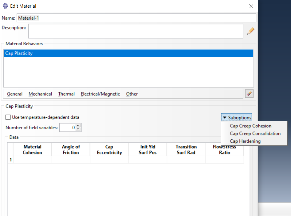
Figure 8: Cap Plasticity model in Abaqus

Concrete Damaged Plasticity Model

The Concrete Damaged Plasticity (CDP) model is designed to simulate the inelastic behavior of concrete and other quasi-brittle materials. It accounts for the degradation of stiffness due to cracking and crushing, capturing both tensile cracking and compressive crushing phenomena.

The stress-strain relation for the general three-dimensional multiaxial condition is defined as:

Where:

• σ is the stress tensor
• D is scalar damage variable (0 ≤ d ≤ 1)
• D_el is elastic stiffness tensor
•  is the total strain tensor
•  is the plastic strain tensor

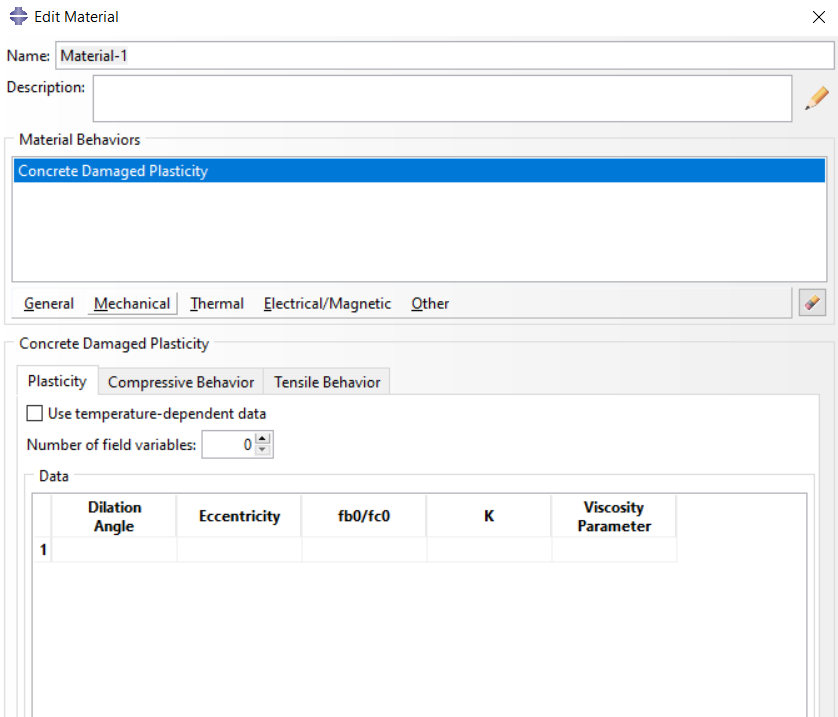
Figure 9: Concrete Damage Plasticity model in Abaqus

This model is available in the Property module as you can see in the next figure. If you want to know more about this model you can refer to our blog “Concrete Damage Plasticity (CDP) in Abaqus”.

Soil Impact Analysis Using Coupled Eulerian-Lagrangian (CEL) Method

The Coupled Eulerian-Lagrangian (CEL) approach in Abaqus is designed to handle problems involving extreme deformations, where traditional Lagrangian methods may fail due to mesh distortion. In soil mechanics, CEL is particularly useful for simulating scenarios such as:

• Penetration of objects into the soil (e.g., pile driving, anchor embedding)
• Explosive interactions with soil
• Large deformation problems like landslides or debris flows

By combining Eulerian and Lagrangian formulations, CEL allows the soil (modeled with Eulerian elements) to flow through a fixed mesh, while the structure (modeled with Lagrangian elements) can move and deform freely. Unlike the previous cases, CEL is a modeling method, not a damage model. Therefore, when using this modeling method, various damage models can also be used.

Note: You can learn all about CEL method, what is this method, learn the theory, and how to implement it in Abaqus in our latest blog: “Coupled Eulerian Lagrangian Full Guide + Abaqus Simiulation Tips“

Abaqus Geotechnical Applications

Abaqus geotechnical modeling is widely applied in various geotechnical engineering analyses. Typical Abaqus geotechnical applications include:

• Geostatic analysis for in-situ stress initialization
• Soil–structure interaction in shallow and deep foundations
• Slope stability and embankment analysis
• Consolidation and pore pressure dissipation
• Seismic geotechnical analysis and liquefaction modeling

These capabilities make Abaqus a reliable finite element tool for advanced geotechnical simulations.

Conclusion

This article focused on Abaqus soil modeling. It introduced different Abaqus soil models and methods used in geotechnical engineering analysis. Simulating soil correctly is important because soil behavior affects the stability and safety of structures, especially under loads, settlement, or seismic activity.

We started by discussing why soil modeling matters and how Abaqus helps simulate real soil responses. Then, we explained key Abaqus soil models: the Mohr-Coulomb model for granular materials, the Clay Plasticity model for cohesive soils, and the Drucker-Prager model for smooth and stable simulations. We also covered the Cap Plasticity model, useful for pressure-dependent materials, and the Concrete Damaged Plasticity model, which is relevant when soil interacts with concrete elements.

Finally, we introduced the CEL method, which handles large deformation problems like penetration or landslides. Overall, this article showed that using the right model or method in Abaqus helps engineers better understand and predict how soil will behave in real projects.

Overall, Abaqus geotechnical modeling provides a robust numerical framework for solving complex soil and geotechnical engineering problems with high accuracy.

[/vc_column_text][/vc_column][/vc_row]

The CAE Assistant is committed to addressing all your CAE needs, and your feedback greatly assists us in achieving this goal. If you have any questions or encounter complications, please feel free to share it with us through our social media accounts including WhatsApp.

Explore our comprehensive Abaqus tutorial page, featuring free PDF guides and detailed videos for all skill levels. Discover both free and premium packages, along with essential information to master Abaqus efficiently. Start your journey with our Abaqus tutorial now!