
")
")


Abaqus convergence tutorial | Introduction to Nonlinearity and Convergence in ABAQUS
€ 120.0
This package introduces nonlinear problems and convergence issues in Abaqus. Solution convergence in Abaqus refers to the process of refining the numerical solution until it reaches a stable and accurate state. Convergence is of great importance especially when your problem is nonlinear; So, the analyst must know the different sources of nonlinearity and then can decide how to handle the nonlinearity to make solution convergence. Sometimes the linear approximation can be useful, otherwise implementing the different numerical techniques may lead to convergence.
Through this tutorial, different nonlinearity sources are introduced and the difference between linear and nonlinear problems is discussed. With this knowledge, you can decide whether you can use linear approximation for your nonlinear problem or not. Moreover, you will understand the different numerical techniques which are used to solve nonlinear problems such as Newton-Raphson.
All of the theories in this package are implemented in two practical workshops. These workshops include modeling nonlinear behavior in Abaqus and its convergence study and checking different numerical techniques convergence behavior using both as-built material in Abaqus/CAE and UMAT subroutine.
| Expert | |
|---|---|
| Package Content |
.inps,video files, Fortran files (if available), Flowchart file (if available), Python files (if available), Pdf files (if available) |
| Tutorial video duration |
90 Minutes |
| language |
English |
| Level | |
| Package Type | |
| Software version |
Applicable to all versions |
| Subtitle |
English |
Frequently Bought Together
Abaqus convergence tutorial
Mastering convergence is crucial for getting accurate results from your Abaqus simulations, especially when dealing with nonlinear problems. This Abaqus convergence tutorial dives deep into the theory behind convergence and equips you with the skills to tackle it. You’ll learn how to identify different sources of nonlinearity and explore how they impact convergence. The practical workshops will guide you through simulating nonlinear behavior and investigating the convergence behavior of various numerical techniques, like Newton-Raphson and Quasi-Newton. By the end, you’ll be confident in achieving stable and reliable solutions for your complex Abaqus analyses.
Introduction
Most engineers and scientists studying physical phenomena are involved with two major tasks:
- Mathematical formulation of the physical process
- Numerical analysis of the mathematical model
Among the different numerical methods, Finite Element Method (FEM) has become an essential tool for engineers and designers as it offers numerous benefits and advantages over traditional methods of problem-solving. These advantages include:
- Accurate and Precise Results
- Time-Saving
- Cost-Effectiveness
- Versatility
- Optimization
- Future-Proofing
Abaqus is a powerful finite element analysis (FEA) software that can be used to solve a wide variety of engineering problems. These problems can range from simple linear problems, such as calculating the stress in a beam under a load, to complex nonlinear problems, such as simulating the collapse of a building under an earthquake.
Nonlinear problems in Abaqus encompass a wide range of physical phenomena that exhibit a departure from linear behavior. These problems involve material or system responses that are not proportional to the applied loads, resulting in complex and often unpredictable outcomes.
In Abaqus, nonlinear problems are characterized by material properties or boundary conditions that vary with deformation, load magnitude, or other parameters.
One of the critical aspects of using Abaqus is ensuring the convergence of the solution, which is the process of reaching a stable and accurate result. In Abaqus, convergence is typically measured by monitoring the residuals of the governing equations, such as the force balance and the displacement equilibrium. The residuals represent the imbalance in the equations and should decrease as the solution converges. Here we want to provide a comprehensive understanding of solution convergence in Abaqus and its importance. (Abaqus convergence tutorial)
What is Convergence in FEA?
Solution convergence in Abaqus is a critical aspect of numerical simulation to ensure the accuracy and reliability of the results. Convergence refers to the process by which the solution approaches a consistent and stable value as the simulation progresses.
In FEA “convergence” can imply multiple meanings such as:
• Mesh convergence
• Time integration accuracy
• Convergence of nonlinear solution procedure
• Solution accuracy
Each one of these convergence meanings is completely discussed in this chapter. (Abaqus convergence tutorial)(Abaqus convergence tutorial)(Abaqus convergence tutorial)(Abaqus convergence tutorial)
What is a Nonlinear problem?
Nonlinear problems are those in which the material behavior or the loading conditions are not linear. This means that the relationship between stress and strain is not a straight line, or that the loading conditions vary throughout the analysis.
Nonlinear problems are an important part of engineering analysis. Abaqus provides a powerful set of tools that can be used to solve a wide variety of nonlinear problems. By understanding the different types of nonlinear problems and the tools available in Abaqus, users can successfully solve even the most complex nonlinear problems.
There are three common sources of nonlinearity:
- Geometry
These arise when the deformation of a structure significantly alters its geometry, affecting the load paths and deformation patterns. For example, the buckling of a slender beam or the large-scale deformation of a soft tissue.
- Material
These involve materials with stress-strain relationships that are nonlinear, such as plastic deformation of metals, creep of polymers, or strain softening of concrete.
- Boundary
Occurring when surfaces interact, leading to complex contact forces and deformation patterns. These are often encountered in simulations involving friction, impact, or assembly processes.
Various types of nonlinearities will be discussed through simple examples in this chapter.
Properties of Linear and Nonlinear Problems
Linear and nonlinear problems are two broad categories of mathematical and scientific problems that are encountered in various fields such as physics, engineering, economics, and computer science. The distinction between these two types of problems lies in the nature of the relationships between the variables involved. Understanding the properties of linear and nonlinear problems is crucial for selecting appropriate methods and techniques to solve them.
Linear problems have the following features:
- Existence
For each load F there will always be at least one solution u.
- Uniqueness
For each F there will always be only one solution u!
- Scaling
If F causes a displacement u, then aF causes a displacement au.
- Superposition
If F causes a displacement u and G causes a displacement v, then F + G causes a displacement u + v.
Nonlinear problems have the exact opposite features and an additional one:
- History Dependent
In a nonlinear problem, the “unique” solution u at time t is determined by the entire load history of P(t).
Numerical Techniques for Solving Nonlinear Problems
Numerical methods offer efficient and reliable approaches to obtaining accurate solutions for complex systems and scenarios. These techniques provide approximate numerical solutions to nonlinear problems, where analytical solutions may not be readily available. Two of the most common techniques discussed in this chapter:
- Newton-Raphson method
The Newton-Raphson method is a popular iterative technique for finding the roots of a nonlinear equation. The method is based on the idea of approximating the function with a linear function at each iteration and then using the linear approximation to find a better estimate of the root. The process continues until the desired level of accuracy is achieved. Newton’s method is particularly useful for solving nonlinear equations with a single variable, and it converges rapidly when the initial guess is close to the actual root. (Abaqus convergence tutorial)
- Quasi-Newton method
Quasi-Newton methods are a class of optimization algorithms that approximate the Hessian matrix of the function using only first-order information. The method involves iteratively updating the Hessian approximation and using it to find a better estimate of the minimum. Quasi-Newton methods are particularly useful for solving large-scale optimization problems, as they can handle non-differentiable functions and do not require the computation of second-order derivatives.
Implementing these methods in Abaqus simulations (Abaqus convergence tutorial) is covered in this chapter and the workshops of this package.
Workshop 1: Nonlinear Behavior | Nonlinear spring modeling
In this workshop, first, you will learn how to simulate a nonlinear spring in Abaqus/CAE. A nonlinear spring is the one whose force-displacement diagram is not linear and its stiffness changes during loading; it can have either a hardening behavior or softening. Because the model is nonlinear, convergence is an issue. So, the solution convergence is also checked in the simulation. The effect of time increment is also considered both on the convergence and the behavior of the model. (Abaqus convergence tutorial)
Workshop 2: Numerical Techniques Convergence
In this workshop, a plate under uniaxial tension is modeled. The load in this model is applied via two different methods: load control and displacement control. The main goal of this workshop is to investigate the effect of numerical techniques used to solve the problem on solution convergence. Different numerical techniques including Newton-Raphson and Quasi-Newton are compared and the effect of the tangent matrix on convergence is discussed. The tangent matrix effect on convergence is studied by changing this matrix once by using the Quasi-Newton method and once by using a user material subroutine (UMAT).
This workshop will provide you with great information about different numerical techniques and their convergence rate.
If you want to know about convergence issues and how to solve them, this article could be a great start (Abaqus convergence tutorial): “Abaqus convergence issues in simple terms | FEA convergence problem“.
It would be helpful to see Abaqus Documentation to understand how it would be hard to start an Abaqus simulation without any Abaqus tutorial. Moreover, if you need to get some info about the FEM, visit this article: “Introduction to Finite Element Method | Finite Element Analysis”.
One note, when you are simulating in Abaqus, be careful with the units of values you insert in Abaqus. Yes! Abaqus don’t have units but the values you enter must have consistent units. You can learn more about the system of units in Abaqus.
Also, learn about: Automatic Stabilization Abaqus of Unstable Problems
Read More: What is Abaqus Small Sliding? | Finite Sliding VS Small Sliding
Read More: What is Abaqus Contact Damping and how to apply it in Abaqus?
All the package includes Quality assurance of training packages. According to this guarantee, you will be given another package if you are not satisfied with the training, or your money is returned. Get more information in terms and conditions of the CAE Assistant.
All packages include lifelong support, 24/7 support, and updates will always be sent to you when the package is updated with a one-time purchase. Get more information in terms and conditions of the CAE Assistant.
Notice: If you have any question or problem you can contact us.
Ways to contact us: WhatsApp/Online Support/Support@CAEassistant.com/ contact form.
Projects: Need help with your project? You can get free consultation from us here.
To access tutorial video run the .exe file on your personal pc and send the generated code to shop@caeassistat.com and wait for your personal code, which is usable only for that pc, up to 24 hours from CAE Assistant support.
Here you can see the purchase process of packages: Track Order
You must be logged in to post a review.
You may also like…
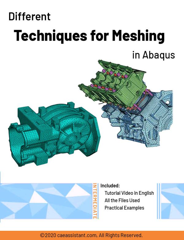

Different Techniques for Meshing in Abaqus


ABAQUS course for beginners | FEM simulation tutorial
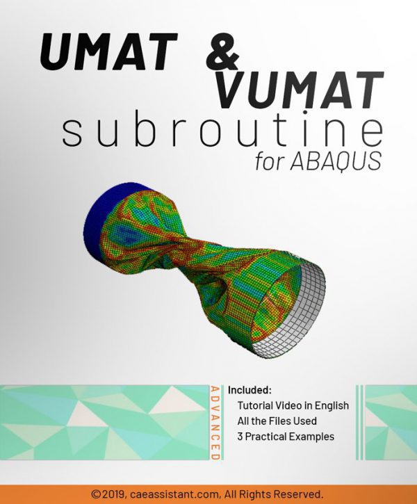

UMAT Subroutine (VUMAT Subroutine) introduction
This package is usable when the material model is not available in ABAQUS software. If you follow this tutorial package, including standard and explicit solver, you will have the ability to write, debug and verify your subroutine based on customized material to use this in complex structures. These lectures are an introduction to write advanced UMAT and VUMAT subroutines in hyperelastic Martials, Composites and Metal and so on.
Watch Demo
Reviews
Clear filtersThere are no reviews yet.